Download
1 / 30
320 likes | 481 Views
This lecture covers key concepts in information theory, including entropy, source coding, channel coding, and multi-user models. Topics include constraint sequences, cryptography applications, and different channel models such as the binary symmetric channel. The lecture explores channel capacity, errors, interleaving, and decoding methods. Examples of Middleton's Class A channel models are discussed, along with their parameters and capacity calculations. Homework assignments and theoretical concepts related to channel capacity and coding methods are also included.

E N D
Introduction to Information theorychannel capacity and models A.J. Han Vinck University of Essen October 2002
content • Introduction • Entropy and some related properties • Source coding • Channel coding • Multi-user models • Constraint sequence • Applications to cryptography
This lecture • Some models • Channel capacity • converse
some channel models Input X P(y|x) output Y transition probabilities memoryless: - output at time i depends only on input at time i - input and output alphabet finite
channel capacity: I(X;Y) = H(X) - H(X|Y) = H(Y) –H(Y|X)(Shannon 1948) H(X) H(X|Y) notes: capacity depends on input probabilities because the transition probabilites are fixed X Y channel
channel model:binary symmetric channel • 1-p • 0 0 • p • 1 • 1-p Error Source E X + Output Input E is the binary error sequence s.t. P(1) = 1-P(0) = p X is the binary information sequence Y is the binary output sequence
burst error model Random error channel; outputs independent P(0) = 1- P(1); Error Source Burst error channel; outputs dependent P(0 | state = bad ) = P(1|state = bad ) = 1/2; P(0 | state = good ) = 1 - P(1|state = good ) = 0.999 Error Source State info: good or bad transition probability Pgb Pbb Pgg good bad Pbg
Interleaving: bursty Message interleaver channel interleaver -1 message encoder decoder „random error“ Note: interleaving brings encoding and decoding delay Homework: compare the block and convolutional interleaving w.r.t. delay
Interleaving: block Channel models are difficult to derive: - burst definition ? - random and burst errors ? for practical reasons: convert burst into random error read in row wise transmit column wise 1 0 0 1 1 0 1 0 0 1 1 0 000 0 0 1 1 0 1 0 0 1 1
De-Interleaving: block read in column wise this row contains 1 error 1 0 0 1 1 0 1 0 0 1 1 e e e e e e 1 1 0 1 0 0 1 1 read out row wise
Interleaving: convolutional input sequence 0 input sequence 1 delay of b elements input sequence m-1 delay of (m-1)b elements Example:b = 5, m = 3 in out
Class A Middleton channel model AWGN, σ20 I Q I Q AWGN, σ21 … AWGN, σ22 I and Q same variance … Select channel k with probability Q(k) 0 1 0 1 Transition probability P(k)
Example: Middleton’s class A Pr{ σ =σ(k) } = Q(k), k = 0,1, · · · A is the impulsive index are the impulsive and Gaussian noise power
Example of parameters • Middleton’s class A= 1; E = σ = 1; σI /σG = 10-1.5 k Q(k)p(k) (= transitionprobability ) 0 0.36 0.00 1 0.37 0.16 2 0.19 0.24 3 0.06 0.28 4 0.02 0.31 Average p = 0.124; Capacity (BSC) = 0.457
Example of parameters 0 1 0 1 Middleton’s class A: E = 1; σ = 1; σI /σG = 10-3 Transition probability P(k) 1 0.5 0.0 1 0.5 0.0 1 0.5 0.0 Q(k) Q(k) Q(k) 0.5 0.5 0.5 p(k) p(k) p(k) A = 0.1 A = 1 A = 10
Example of parameters 0 1 0 1 Middleton’s class A: E = 0.01; σ = 1; σI /σG = 10-3 Transition probability P(k) 1 0.5 0.0 1 0.5 0.0 1 0.5 0.0 Q(k) Q(k) Q(k) 0.5 0.5 0.5 p(k) p(k) p(k) A = 0.1 A = 1 A = 10
channel capacity: the BSC I(X;Y) = H(Y) – H(Y|X) the maximum of H(Y) = 1 since Y is binary H(Y|X) = h(p) = P(X=0)h(p) + P(X=1)h(p) • 1-p • 0 0 • p • 1 • 1-p X Y Conclusion: the capacity for the BSC CBSC = 1- h(p) Homework: draw CBSC , what happens for p > ½
channel capacity: the Z-channel Application in optical communications H(Y) = h(P0 +p(1- P0 ) ) H(Y|X) = (1 - P0 ) h(p) For capacity, maximize I(X;Y) over P0 0 1 0 (light on) 1 (light off) X Y p 1-p P(X=0) = P0
channel capacity: the erasure channel Application: cdma detection 1-e e e 1-e I(X;Y) = H(X) – H(X|Y) H(X) = h(P0 ) H(X|Y) = e h(P0) Thus Cerasure = 1 – e (check!, draw and compare with BSC and Z) 0 1 0 E 1 X Y P(X=0) = P0
channel models: general diagram P1|1 y1 x1 P2|1 Input alphabet X = {x1, x2, …, xn} Output alphabet Y = {y1, y2, …, ym} Pj|i = PY|X(yj|xi) In general: calculating capacity needs more theory P1|2 y2 x2 P2|2 : : : : : : xn Pm|n ym
clue: I(X;Y) is convex in the input probabilities i.e. finding a maximum is simple
Channel capacity Definition: The rate R of a code is the ratio , where k is the number of information bits transmitted in n channel uses Shannon showed that: : for R C encoding methods exist with decoding error probability 0
System design Code book Code word in receive message estimate 2k decoder channel Code book n There are 2k code words of length n
Channel capacity: sketch of proof for the BSC Code: 2k binary codewords where p(0) = P(1) = ½ Channel errors: P(0 1) = P(1 0) = p i.e. # error sequences 2nh(p) Decoder: search around received sequence for codeword with np differences space of 2n binary sequences
Channel capacity: decoding error probability • For t errors: |t/n-p|> Є • 0 for n (law of large numbers) 2. > 1 code word in region (codewords random)
Channel capacity: converse For R > C the decoding error probability > 0 Pe k/n C
Converse: For a discrete memory less channel channel Xi Yi Source generates one out of 2k equiprobable messages source encoder channel decoder m Xn Yn m‘ Let Pe = probability that m‘ m
converse R := k/n k = H(M) = I(M;Yn)+H(M|Yn) Xn is a function of M Fano I(Xn;Yn) +1+ k Pe nC +1+ k Pe 1 – C n/k - 1/k Pe Pe 1 – C/R - 1/k Hence: for large k, and R > C, the probability of error Pe > 0
Appendix: Assume: binary sequence P(0) = 1 – P(1) = 1-p t is the # of 1‘s in the sequence Then n , > 0 Weak law of large numbers Probability ( |t/n –p| > ) 0 i.e. we expect with high probability pn 1‘s
Appendix: Consequence: 1. 2. 3. 4. n(p- ) < t < n(p + ) with high probability A sequence in this set has probability