Download
1 / 30
300 likes | 384 Views
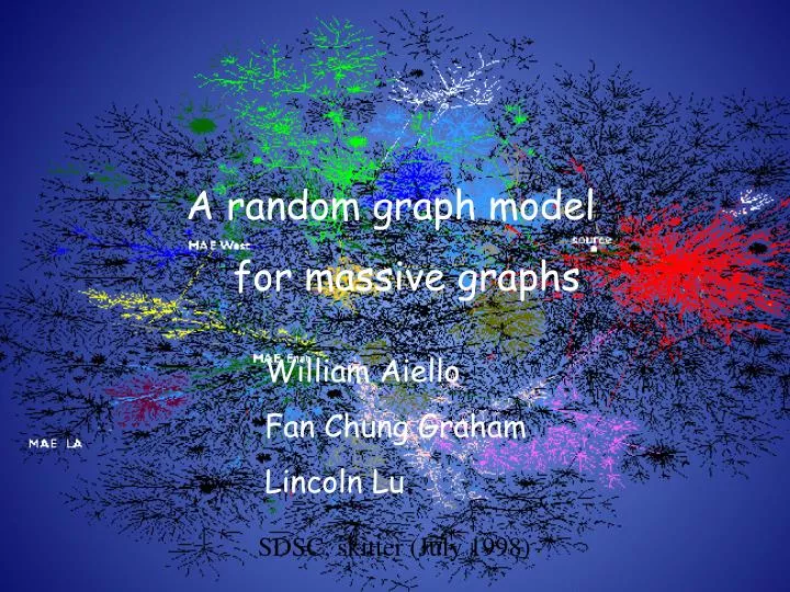
A random graph model for massive graphs. William Aiello Fan Chung Graham Lincoln Lu. SDSC, skitter (July 1998). What are the properties of the WWW Graph?. Is the World Wide Web connected? If not, how large is the largest component, the second largest component, etc.?

E N D
A random graph model for massive graphs William Aiello Fan Chung Graham Lincoln Lu SDSC, skitter (July 1998)
What are the properties of the WWW Graph? • Is the World Wide Web connected? • If not, how large is the largest component, the second largest component, etc.? • Can these questions be answered exactly? • Probably not! The WWW is changing constantly. Even a “snapshot” of the Web is too large to handle.
An important observation Discovered by several groups independently • Broder, Kleinberg, Kumar, Raghavan, Rajagopalan aaand Tomkins, 1999. • Barabási, Albert and Jeung, 1999. WWW graph has a power law degree distribution
Power Law Graphs Power law decay of the degree distribution: The number of vertices of degree d is proportional to 1/db where b is some constant > 0. Let y(d) be the number of nodes of degree d y ~ 1/db log y = a – blog d
Power Law Graphs Robust and Ubiquitous • Internet Router Graph • Power Grid Graph • Phone Call Graph • Scientific Citation Graph • Co-Stars Graph (e.g. the six degrees of Kevin Bacon) • The power in the power law stays constant even as the graphs grow and change.
What does a massive graph look like? sparse clustered small diameter prohibitively large dynamically changing incomplete information Hard to describe ! Harder to analyze !!
Don’t worry about exact answers—Use Models Instead • Data sets too large and dynamic for exact analysis occur in many other areas: the physical, biological, and social sciences and engineering. • Progress in understanding often made by iterative interplay between modeling and experimental data, where both often have a random or statistical nature.
Modeling Power Law Graphs • Develop model of Power Law Graphs • Analyze properties of model, e.g., connected component structure • Compare results to experimental data • Our model will be of variant of an important model in graph theory called Random Graphs
Random Graphs • G(n,e) • n nodes • all graphs with e edges have uniform probability H(3,1) prob 1/3 H(3,2) prob 1/3
Random Graphs • G(n,p) • n nodes • each edge is included with probability p • expected degree = p(n-1) p(1-p)2 (1-p)3 p3 p2(1-p)
.. / Paul Erdos and A. Renyi, On the evolution of random graphs Magyar Tud. Akad. Mat. Kut. Int. Kozl. 5 (1960) 17-61.
The evolution of random graphs G(n,p) 0 disjoint union of trees c/n, 0<c<1 cycles of any size 1/n the double jumps p c’/n, c>1 one giant component, i.e., size (n), other components are o(n)-sized trees log n/n G(n,p) is connected w log n/n, w connected and almost regular, expected degree ~ w log n
Random Graphs and Degree Distributions • H(n,s) • n nodes • s = (y(1), y(2), … , y(n-1)), where y(i) is the number of nodes with degree i. • all graphs with degree distribution s have uniform probability
Random Graphs and Degree Distributions H(4,s), s = (1,2,1). All have prob. 1/12
Random Power Law Graphs A power law degree distribution can be described by two parameters: a, b y = ea/xb log y = a – b log x where y is the number of nodes of degree x A new random graph model: P(a,b). P(a,b) assigns uniform probability to all graphs with degree distribution y = ea/xb
A few facts about P(,): • The maximum degree is e/. • The number of vertices n is • n = e/x~ z() e , 1 x ea/b, • where z(b) = S1/xb the Reimann Zeta function. • The number of edges E is • E = 1/2 e/x-1~ z(-1) e/2 • The density E/n = z(b-1)/z(b) is controlled by b.
Facts on P(,): 0 connected 1 not connected—unique giant component of size (n) smaller components are of size O(1). 2 smaller components are of size O(log n/log log n). For any x, 2<≤x<O(log n/log log n), there is a component of size x. The second largest components are of size O(log n). For any x, 2<x<O(log n), there is a component of size x. a root of ς(-2)=2 ς(-1) 3.478... no giant component
How do Power Law Graphs Arise? • The previous model takes the power law degree distribution as a given. • It does not explain how such graphs arise. • Results which hold in the model with high probability (e.g., our connected component results) will apply to the vast majority of power law graphs regardless of the particulars of the evolution process.
Yet Another Random Graph Model G(n) is a random graph evolution: • Let Kn be the set of all possible edges • Let Et be the edges chosen in steps 1 through t. • At time step t+1 choose uniformly one of the edges in Kn – Et • Add this edge to Et to get Et+1. • Study what structures appear with high probability as a function of t.
Need a new idea • G(n) fixes the set of nodes and then adds edges. • Can show that to get a power law, need to add both nodes and edges. • G(n) chooses uniformly among all eligible edges • Can show that selecting edges uniformly will not yield a power law.
A Graph Evolution Process • At each time step t, toss a biased coin having heads with probability p. • “tails” -> add a new vertex with a self-loop. • “heads” -> add a new edge between the existing set of nodes: • Select a vertex u with probability proportional to the the degree of u, i.e., Pr[ u chosen ] = deg(u)/2|E|. • Independently select vertex v with probability proportional to deg v. • Add the edge {u,v}.
p 1-p v Gt u A Graph Evolution Process • The number of nodes grows with time • Edges are not added uniformly • Nodes which are added early have an “advantage” over nodes added late • Gives a power law degree distribution y ~ 1/d1+1/p
Comparisons From simulation using Model B From real data
Evolution Process for Directed Graphs • Select a vertex u with probability proportional to the the out degree of u, i.e., Pr[ u chosen ] = out-deg(u)/|E|. • Select a vertex v with probability proportional to the the in degree of v. • Flip two coins; heads with prob p1 and p2. • Heads, heads -> add an edge from u to v. • Heads, tails -> add an edge from u to a new node. • Tails, heads -> add an edge from a new node to v. • Tails, Tails -> add a directed self-loop to a new node. • # nodes w/outdegree d ~ 1/d1+1/p1 • # nodes w/indegree of d ~ 1/d1+1/p2
Massive Graphs Random graphs Similarities: Adding one (random) edge at a time. Differences: Random graphs <-- almost regular. Massive graphs <-- uneven degrees. Correlations.
The advantages of power law models • Approximating real data graphs. • Possible to analyze rigorously—discover implicit structure of massive graphs • Models for generating network topologies
Methods: • Erdös and Réyni’s seminal papers. • Martingales. • Concentration bounds. • Molloy+Reed’s results on random graphs with.given degree squences.
Future directions The evolution of power graphs concerning ---- diameters of connected components luuuuuuuuuuuuuuuuuuuuuuuuuuuuuuuuuuuuuuLu’sthesis -- - frequency of occurrences of certain subgraphs - power law of eigenvalues - scaling behavior of power law graphs - “signatures” in graphs to distinguish models A JAVA generation/simulation of power graphs Can be found at http://math.ucsd.edu/~llu