Download
1 / 20
200 likes | 391 Views
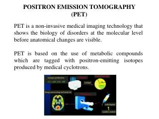
Time of Flight in Positron Emission Tomography using Fast Sampling. Dan Herbst Henry Frisch. Summary. Overview of PET Fast sampling capabilities Experimental setup Data Analysis. PET. Metabolically-active positron tracer Antiparallel 511 kEv photon emission Detector ring.

E N D
Time of Flight in Positron Emission Tomography using Fast Sampling Dan Herbst Henry Frisch
Summary • Overview of PET • Fast sampling capabilities • Experimental setup • Data • Analysis
PET • Metabolically-active positron tracer • Antiparallel 511 kEv photon emission • Detector ring http://www.scq.ubc.ca/looking-inside-the-human-body-using-positrons/
Fast Sampling • Tektronix • 40 Gs/sec • $142K retail • Continuous fast sampling • BLAB1 • ~5.12 Gs/sec • ~$10/channel in bulk • Triggered burst of fast sampling
Hardware Work • Uploaded drivers onto BLAB’s FPGA • Plateaued tubes • Setup coincidence detection • Setup delay lines to BLAB • Collected data
Data • Oscilloscope & BLAB pulses (different event)
Filtering on Energy • Many photons will Compton scatter off of scintillation crystal, only depositing partial energy • Keep only events where both pulses are fully absorbed
Pulse Smoothing • Experimented with different algorithms • Ended up using: f(t) such that is minimized. • Parameter ‘c’ determines smoothness
A Typical Time Extraction Algorithm • Fit the leading-edge points to a function (i.e. linear fit), and take where that function crosses the baseline Qingguo Xie, UChicago Department of Radiology
My Objections • Why weight all points on the leading edge equally? • Why fit to a line or other arbitrary function? • Make these things parameters and feed to an optimization algorithm • Quality measure: standard deviation of timing difference over a large set of representative pulse pairs
Why Pulse Shape Optimizations May Have Failed in the Past • Many degrees of freedom • Valleys become narrow, must scale parameters • Time extraction must be fast to give optimizer many attempts • Bias in stepping unless careful
My Timing Extractor • Normalize pulses • Fit the template to the pulse under the transformations: • Time shift • Time scale (about a given point) • y-scale (optional) • …using least squares (horizontal!)
Advantage • Since least squares fitting is in horizontal direction, time-shift, time-scale, and scale-about point (global) are calculated analytically Disadvantage • Pulse is only “sampled” at a limited number of points • Working on a new version to fix this problem
Results (scope data) • ~300 p.s. FWHM without y-scaling • ~270 p.s. with y-scaling (need to confirm)
Results (BLAB data) • 957 p.s. FWHM assuming 5.12 Gs/sec • Obviously there was a malfunction somewhere
Where to Proceed • Short term: • Shorten travel distances in photo-tube base • Finish full-sampling version of pulse-shape optimizer • Understand BLAB results • Long term: • Simulate and optimize phototube design • Improve fast sampling board
How does Time of Flight improve tumor detection? Slide by Joel Karp, University of Pennsylvania Dept. of Radiology & Physics March 27, 2008 nonTOF #iter = 10 scan time = 5 min 3 min 2 min 1min TOF #iter = 5 35-cm diameter phantom 10, 13, 17, 22-mm hot spheres (6:1 contrast); 28, 37-mm cold spheres background activity concentration of 0.14 Ci/ml TOF achieves better contrast, with shorter scan