Download

1 / 56
560 likes | 681 Views
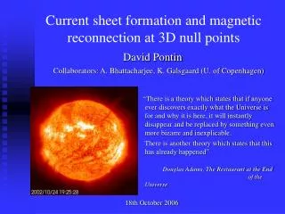
Current sheets formation along magnetic separators in 3d. Dana Longcope Montana State University. Thanks: I Klapper, A.A. Van Ballegooijen NSF-ATM. The Coronal Field. 8/11/01 9:25. 1 MK plasma (TRACE 171A). Corona : complex inter-connections between sources. B z =0. Lower boundary :

E N D
Current sheets formation along magnetic separators in 3d Dana Longcope Montana State University Thanks: I Klapper, A.A. Van Ballegooijen NSF-ATM
The Coronal Field 8/11/01 9:25 1 MK plasma (TRACE 171A) Corona: complex inter-connections between sources Bz=0 Lower boundary: Bz confined to source regions 8/10/01 12:51 Magnetic field @ photosphere (MDI)
The Coronal Field 8/11/01 9:25 1 MK plasma (TRACE 171A) Evolution: lower boundary changes slowly 8/10/01 12:51 8/11/01 17:39 Magnetic field @ photosphere (MDI) (+30 hrs)
Outline I. Lowest energy magnetic field contains current sheets localized to separators (Flux-Constrained Equilibrium) II. Boundary motion drives field singular equilibrium via repeated Alfven wave reflection
I. Equilibrium Force-Free Equilibrium: Minimizes Mag. Energy* *subject to BC: Bz(x,y,0) = f(x,y) • Constraints: (minimize subject to…) • None • Ideal motion (line-tied to boundary) potential general FFF
A new type of constraint (Longcope 2001, Longcope & Klapper 2002) Bz=0 Boundary field Bz(x,y,0) = f(x,y): assumediscrete sources
A new type of constraint Constrain coronal flux interconnecting sources The domain graph P1 N4 P2 N5 N6 P3 Summarizes the Magnetic connectivity
Structure of Constraint • Domain D16 connects P1 N6 • Flux in Domain D16: y16 (want to specify this) • Flux in source 6: F6 (set by BC) P1 N4 P2 N5 N6 P3
Structure of Constraint • Domain D16 connects P1 N6 • Flux in Domain D16: y16 (want to specify this) • Flux in source 6: F6 (set by BC) • Inter-related through incidence matrix of graph: i.e. -y16 - y26 - y36 =F6 P1 N4 P2 N5 N6 P3
Structure of Constraint Q: How many domain fluxes yab may be independantly specified? P1 N4 A: Nc = Nd – Ns + 1 P2 N5 N6 P3 Number of domains Number of sources here Nc = 7 – 6 + 1 = 2
Structure of Constraint Q: How many domain fluxes yab may be independantly specified? y14=Y2 P1 N4 y34=Y1 A: Nc = Nd – Ns + 1 P2 N5 Specifying fluxes of Ncchords reduces graph to a tree N6 P3
Structure of Constraint Q: How many domain fluxes yab may be independantly specified? y14=Y2 P1 N4 y34=Y1 A: Nc = Nd – Ns + 1 P2 N5 Specifying fluxes of Ncchords reduces graph to a tree… all remaining fluxes follow from flux balance: y36=F3-Y1 … etc. N6 P3
How to apply constraints • Topology of the • potential field:* • Extrapolate from • bndry: • Locate all magnetic • null points B=0 • Trace spine field lines • to spine sources *same topology will apply to non-potential fields
The skeleton of the field • Trace all fan field • lines from null • Form sectors • Joined at • separators • A separator • connects + - • null points
The skeleton of the field • Trace all fan field • lines from null • Form sectors • Joined at • separators • A separator • connects + - • null points
The skeleton of the field • Trace all fan field • lines from null • Form sectors • Joined at • separators • A separator • connects + - • null points
The skeleton of the field • Trace all fan field • lines from null • Form sectors • Joined at • separators • A separator • connects + - • null points
Individual Domains Domain linking PaNb must be bounded by sectors +’ve sectors: Pa @ apex -’ve sectors: Nb @ apex Sectors intersect @closed separator circuit Circuit encircles domain
Formulating the constraint P1 N4 y34=Y1 P2 N5 N6 P3 Locate separator circuitQiencircling domain Di: Constraint functional:
The Constrained Minimization Lagrange multiplier Minimize: All con- straints Non-potential field: separator curve: Qi annular ribbon xi(x,h) d-function Singular density
The Variation • Vary • Require stationarity: dC = 0 • Get Euler-Lagrange equation Singular current density, confined to separator ribbon i
Flux Constrained Equilibria P1 N4 y23= Y1 • Potential field (w/o constraints): Yi=Yi(v) • Non-potential field: Yi=Yi(v) +DYi i=1,…,Nc • Free Energy in flux-constrained field: • General FFF: P3 N2
Flux Constrained Equilibria • Min’m energy subject to Nc constraints Nc fluxes are parameters:Yi • Current-free within each domain • Singular currents* on all separators P1 N4 P3 N2 Y1 <Y1(v) * Always ideally stable!
II. Approach to Equilibrium (Longcope & van Ballegooijen 2002) • Separator defined through footpoints No locally distinguishing property* • Singularity must build up through repeated reflection of information between footpoints * In contrast to 2 dimensions: B=0 @ X-point
Dynamics Illustrated Sources on end planes Long (almost straight) coronal field (RMHD) Maps between merging layers Equilib. field maps sources to merging layer
Dynamics Illustrated N3 S- N4 Sep’x from null on p-sphere
Dynamics Illustrated N3 N4 Sources move (rotation)
Dynamics Illustrated N3 N4 Sources move (rotation)
Dynamics Illustrated Dq N3 N4 Bf Sources move (rotation) vf Initiates Alfven pulse (uniform rotation)
Dynamics Illustrated Dq N3 N4 Bf Sources move (rotation) vf Initiates Alfven pulse (uniform rotation)
Dynamics Illustrated Dq N3 N4 Bf Sources move (rotation) vf Initiates Alfven pulse (uniform rotation)
Dynamics Illustrated Dq N3 N4 Bf Sources move (rotation) vf Initiates Alfven pulse (uniform rotation)
Dynamics Illustrated Bf vf
Impact at Opposing End P1 S+ P2 c.c rotation Bf Motion at merging height mapped down to photosphere vf
Impact at Opposing End P1 S+ P2 Merging height: No motion across sep’x S+ Free motion w/in source-regions Photosphere: fixed source positions, moveable interiors
Impact at Opposing End c.clockwise motion in each region P1 S+ Vorticity sheet @ sep’x P2 Merging height: No motion across sep’x S+ Free motion w/in source-regions Photosphere: fixed source positions, moveable interiors
Impact at Opposing End P1 N3 S+ S- N4 P2 Image of opposing separator is distorted by boundary motion
Impact at Opposing End P1 N3 S+ S- N4 P2 Image of opposing separator is distorted by boundary motion
Impact at Opposing End P1 N3 S+ S- N4 P2 Image of opposing separator is distorted by boundary motion
Impact at Opposing End P1 N3 S+ S- N4 P2 Intersection of separatrices: The Separator Ribbon
The Reflected Wave P1 S+ P2 Singular Alfven pulse: Voricity/Current sheet confined to S+
The Reflected Wave S+ S- Separator ribbon left in wake of reflection
Repeated Reflection S+ S- z=0 z=L • CS along S+ reflects from z=0 • CS along S- reflects from z=L • Repeated reflection retains only current on • separator ribbon • Wave w/ current on ribbon - perfectly reflected
The Final Current Sheet S+ S- B^ Helical pitch, maps S+ S- z=0 z=L Interior CS (z=0)
The Final Current Sheet S+ S- B^ Helical pitch, maps S+ S- z=0 z=L Interior CS
The Final Current Sheet S+ S- B^ Helical pitch, maps S+ S- z=0 z=L Interior CS
The Final Current Sheet S+ S- B^ Helical pitch, maps S+ S- z=0 z=L Interior CS
The Final Current Sheet S+ S- B^ Helical pitch, maps S+ S- z=0 z=L Flux constrained equilib. I set by e.g y23 Interior CS
Conclusions • New class of constraints: domain fluxes • Flux constrained equilibria have CS on all separators • Equilibrium is approached by repeated Alfven wave reflections from boundary
Implications • Coronal field tends toward singular state • Current sheets are ideally stable • Magnetic reconnection can • Eliminate constraint • Decrease magnetic energy • Free energy depends on flux in NC different fluxes within corona.