Download
1 / 45
450 likes | 556 Views
Required Sample Size, Type II Error Probabilities. Chapter 23 Inference for Means: Part 2. Required Sample Size To Estimate a Population Mean . If you desire a C% confidence interval for a population mean with an accuracy specified by you, how large does the sample size need to be?

E N D
Required Sample Size, Type II Error Probabilities Chapter 23 Inference for Means: Part 2
Required Sample Size To Estimate a Population Mean • If you desire a C% confidence interval for a population mean with an accuracy specified by you, how large does the sample size need to be? • We will denote the accuracy by ME, which stands for Margin of Error.
Example: Sample Size to Estimate a PopulationMean • Suppose we want to estimate the unknown mean height of male students at NC State with a confidence interval. • We want to be 95% confident that our estimate is within .5 inch of • How large does our sample size need to be?
Good news: we have an equation • Bad news: • Need to know s • We don’t know n so we don’t know the degrees of freedom to find t*n-1
A Way Around this Problem: Approximate by Using the Standard Normal
Confidence level Sampling distribution of x .95
Estimating s • Previously collected data or prior knowledge of the population • If the population is normal or near-normal, then s can be conservatively estimated by s range 6 • 99.7% of obs. within 3 of the mean
Example:samplesize to estimate mean height µ of NCSU undergrad. male students We want to be 95% confident that we are within .5 inch of , so • ME = .5; z*=1.96 • Suppose previous data indicates that s is about 2 inches. • n= [(1.96)(2)/(.5)]2 = 61.47 • We should sample 62 male students
Example: Sample Size to Estimate a PopulationMean -Textbooks • Suppose the financial aid office wants to estimate the mean NCSU semester textbook cost within ME=$25 with 98% confidence. How many students should be sampled? Previous data shows is about $85.
Example: Sample Size to Estimate a Population Mean -NFL footballs • The manufacturer of NFL footballs uses a machine to inflate new footballs • The mean inflation pressure is 13.5 psi, but uncontrollable factors cause the pressures of individual footballs to vary from 13.3 psi to 13.7 psi • After throwing 6 interceptions in a recent game, Peyton Manning complains that the balls are not properly inflated. The manufacturer wishes to estimate the mean inflation pressure to within .025 psi with a 99% confidence interval. How many footballs should be sampled?
Example: Sample Size to Estimate a Population Mean • The manufacturer wishes to estimate the mean inflation pressure to within .025 pound with a 99% confidence interval. How may footballs should be sampled? • 99% confidence z* = 2.576; ME = .025 • = ? Inflation pressures range from 13.3 to 13.7 psi • So range =13.7 – 13.3 = .4; range/6 = .4/6 = .067 . . . 1 2 3 48
Hypothesis Testing for , Type II Error Probabilities (Right-tail example) • Example • A new billing system for a department store will be cost- effective only if the mean monthly account is more than $170. • A sample of 400 accounts has a mean of $174 and s = $65. • Can we conclude that the new system will be cost effective?
Example (cont.) • Hypotheses • The population of interest is the credit accounts at the store. • We want to know whether the mean account for all customers is greater than $170. H0 : m = 170 HA : m > 170 • Where m is the mean account value for all customers
Example (cont.) • Test statistic: H0 : m = 170 HA : m > 170
Example (cont.) P-value: The probability of observing a value of the test statistic as extreme or more extreme then t = 1.23, given that m = 170 is… t399 Since the P-value > .05, we conclude that there is not sufficient evidence to reject H0 : =170. Type II error is possible
Calculating , the Probability of aType II Error • Calculating for the t test is not at all straightforward and is beyond the level of this course • The distribution of the test statistic t is quite complicated when H0 is false and HA is true • However, we can obtain very good approximate values for using z (the standard normal) in place of t.
Calculating , the Probability of aType II Error (cont.) • We need to • specify an appropriate significance level ; • Determine the rejection region in terms of z • Then calculate the probability of not being in the rejection when = 1, where 1 is a value of that makes HA true.
Example (cont.) calculating • Test statistic: H0 : m = 170 HA : m > 170 Choose = .05 Rejection region in terms of z: z > z.05 = 1.645 a = 0.05
The rejection region with a = .05. a=.05 H0: m = 170 HA: m = 180 m= 170 m=180 Example (cont.) calculating Express the rejection region directly, not in standardized terms • Let the alternative value be m = 180 (rather than just m>170) Specify the alternative value under HA. Do not reject H0
a=.05 H0: m = 170 H1: m = 180 m= 170 m=180 Example (cont.) calculating • A Type II error occurs when a false H0 is not rejected. Suppose =180, that is H0 is false. A false H0… …is not rejected
H0: m = 170 H1: m = 180 m=180 Example (cont.) calculating Power when =180 = 1-(180)=.9236 m= 170
a2 > b2 < Effects on b of changing a • Increasing the significance level a, decreases the value of b, and vice versa. a1 b1 m= 170 m=180
Judging the Test • A hypothesis test is effectively defined by the significance level a and by the sample size n. • If the probability of a Type II error b is judged to be too large, we can reduce it by • increasing a, and/or • increasing the sample size.
Judging the Test • Increasing the sample size reduces b By increasing the sample size the standard deviation of the sampling distribution of the mean decreases. Thus, the cutoff value of for the rejection region decreases.
m= 170 m=180 Judging the Test • Increasing the sample size reduces b Note what happens when n increases: a does not change, but b becomes smaller
Judging the Test • Increasing the sample size reduces b • In the example, suppose n increases from 400 to 1000. • a remains 5%, but the probability of a Type II drops dramatically.
A Left - Tail Test • Self-Addressed Stamped Envelopes. • The chief financial officer in FedEx believes that including a stamped self-addressed (SSA) envelop in the monthly invoice sent to customers will decrease the amount of time it take for customers to pay their monthly bills. • Currently, customers return their payments in 24 days on the average, with a standard deviation of 6 days. • Stamped self-addressed envelopes are included with the bills for 75 randomly selected customers. The number of days until they return their payment is recorded.
A Left - Tail Test: Hypotheses • The parameter tested is the population mean payment period (m) for customers who receive self-addressed stamped envelopes with their bill. • The hypotheses are:H0: m = 24H1: m < 24 • Use = .05; n = 75.
A Left - Tail Test: Rejection Region • The rejection region: • t < t.05,74 = 1.666 • Results from the 75 randomly selected customers:
A Left -Tail Test: Test Statistic • The test statistic is: Since the rejection region is We do not reject the null hypothesis. Note that the P-value = P(t74< -1.52) = .066. Since our decision is to not reject the null hypothesis, A Type II error is possible.
Left-Tail Test: Calculating , the Probability of a Type II Error • The CFO thinks that a decrease of one day in the average payment return time will cover the costs of the envelopes since customer checks can be deposited earlier. • What is (23), the probability of a Type II error when the true mean payment return time is 23 days?
Left-tail test: calculating (cont.) • Test statistic: H0 : m = 24 HA : m < 24 Choose = .05 Rejection region in terms of z: z < -z.05 = -1.645 a = 0.05
The rejection region with a = .05. m=24 Left-tail test: calculating (cont.) Express the rejection region directly, not in standardized terms • Let the alternative value be m = 23 (rather than just m < 24) H0: m = 24 Specify the alternative value under HA. HA: m = 23 Do not reject H0 a=.05 m= 23
H0: m = 24 HA: m = 23 m=24 Left-tail test: calculating (cont.) Power when =23 is 1-(23)=.282 a=.05 m= 23
A Two - Tail Test for • The Federal Communications Commission (FCC) wants competition between phone companies. The FCC wants to investigate if AT&T rates differ from their competitor’s rates. • According to data from the (FCC) the mean monthly long-distance bills for all AT&T residential customers is $17.09.
A Two - Tail Test (cont.) • A random sample of 100 AT&T customers is selected and their bills are recalculated using a leading competitor’s rates. • The mean and standard deviation of the bills using the competitor’s rates are • Can we infer that there is a difference between AT&T’s bills and the competitor’s bills (on the average)?
A Two - Tail Test (cont.) • Is the mean different from 17.09? • n = 100; use = .05 H0: m = 17.09
a/2 = 0.025 a/2 = 0.025 0 ta/2= 1.9842 -ta/2= -1.9842 Rejection region A Two – Tail Test (cont.) Rejection region t99
0 ta/2= 1.9842 -ta/2= -1.9842 A Two – Tail Test: Conclusion There is insufficient evidence to conclude that there is a difference between the bills of AT&T and the competitor. Also, by the P-value approach: The P-value = P(t < -1.19) + P(t > 1.19) = 2(.1184) = .2368 > .05 a/2 = 0.025 a/2 = 0.025 A Type II error is possible -1.19 1.19
Two-Tail Test: Calculating , the Probability of a Type II Error • The FCC would like to detect a decrease of $1.50 in the average competitor’s bill. (17.09-1.50=15.59) • What is (15.59), the probability of a Type II error when the true mean competitor’s bill is $15.59?
a/2 = 0.025 a/2 = 0.025 Two – Tail Test: Calculating (cont.) Rejection region Do not reject H0 17.09 Reject H0
H0: m = 17.09 HA: m = 15.59 m=17.09 Two – Tail Test: Calculating (cont.) Power when =15.59 is 1-(15.59)=.972 a=.05 m= 15.59
General formula: Type II Error Probability (A) for a Level Test