Download
1 / 39
390 likes | 454 Views
Recall: breadth-first search, step by step. Implementation of search algorithms. Function General-Search(problem, Queuing-Fn) returns a solution, or failure nodes make-queue(make-node(initial-state[problem])) loop do if nodes is empty then return failure

E N D
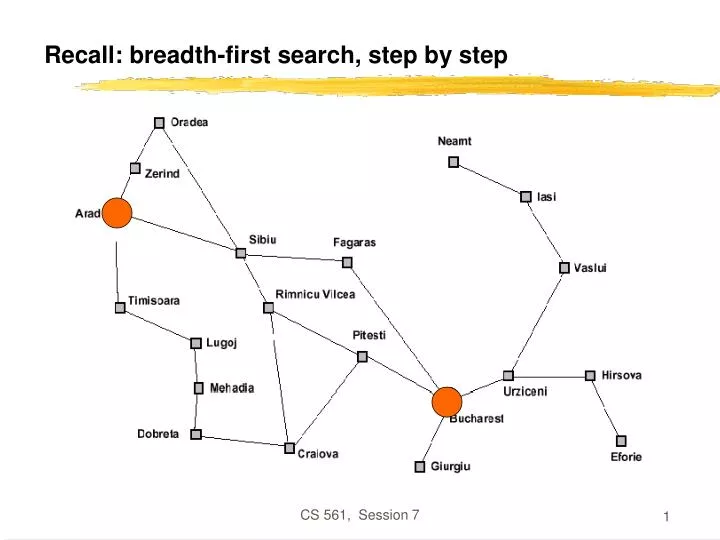
Recall: breadth-first search, step by step CS 561, Session 7
Implementation of search algorithms Function General-Search(problem, Queuing-Fn) returns a solution, or failure nodes make-queue(make-node(initial-state[problem])) loop do if nodes is empty then return failure node Remove-Front(nodes) if Goal-Test[problem] applied to State(node) succeeds then return node nodes Queuing-Fn(nodes, Expand(node, Operators[problem])) end Queuing-Fn(queue, elements) is a queuing function that inserts a set of elements into the queue and determines the order of node expansion. Varieties of the queuing function produce varieties of the search algorithm. CS 561, Session 7
Recall: breath-first search, step by step CS 561, Session 7
Breadth-first search Node queue: initialization # state depth path cost parent # 1 Arad 0 0 -- CS 561, Session 7
Breadth-first search Node queue: add successors to queue end; empty queue from top # state depth path cost parent # 1 Arad 0 0 -- 2 Zerind 1 1 1 3 Sibiu 1 1 1 4 Timisoara 1 1 1 CS 561, Session 7
Breadth-first search Node queue: add successors to queue end; empty queue from top # state depth path cost parent # 1 Arad 0 0 -- 2 Zerind 1 1 1 3 Sibiu 1 1 1 4 Timisoara 1 1 1 5 Arad 2 2 2 6 Oradea 2 2 2 (get smart: e.g., avoid repeated states like node #5) CS 561, Session 7
Depth-first search CS 561, Session 7
Depth-first search Node queue: initialization # state depth path cost parent # 1 Arad 0 0 -- CS 561, Session 7
Depth-first search Node queue: add successors to queue front; empty queue from top # state depth path cost parent # 2 Zerind 1 1 1 3 Sibiu 1 1 1 4 Timisoara 1 1 1 1 Arad 0 0 -- CS 561, Session 7
Depth-first search Node queue: add successors to queue front; empty queue from top # state depth path cost parent # 5 Arad 2 2 2 6 Oradea 2 2 2 2 Zerind 1 1 1 3 Sibiu 1 1 1 4 Timisoara 1 1 1 1 Arad 0 0 -- CS 561, Session 7
Last time: search strategies Uninformed: Use only information available in the problem formulation • Breadth-first • Uniform-cost • Depth-first • Depth-limited • Iterative deepening Informed: Use heuristics to guide the search • Best first: • Greedy search • A* search CS 561, Session 7
Last time: search strategies Uninformed: Use only information available in the problem formulation • Breadth-first • Uniform-cost • Depth-first • Depth-limited • Iterative deepening Informed: Use heuristics to guide the search • Best first: • Greedy search -- queue first nodes that maximize heuristic “desirability” based on estimated path cost from current node to goal; • A* search – queue first nodes that minimize sum of path cost so far and estimated path cost to goal. CS 561, Session 7
This time • Iterative improvement • Hill climbing • Simulated annealing CS 561, Session 7
Iterative improvement • In many optimization problems, path is irrelevant; the goal state itself is the solution. • Then, state space = space of “complete” configurations. Algorithm goal: - find optimal configuration (e.g., TSP), or, - find configuration satisfying constraints (e.g., n-queens) • In such cases, can use iterative improvement algorithms: keep a single “current” state, and try to improve it. CS 561, Session 7
Iterative improvement example: vacuum world Simplified world: 2 locations, each may or not contain dirt, each may or not contain vacuuming agent. Goal of agent: clean up the dirt. If path does not matter, do not need to keep track of it. CS 561, Session 7
Iterative improvement example: n-queens • Goal: Put n chess-game queens on an n x n board, with no two queens on the same row, column, or diagonal. • Here, goal state is initially unknown but is specified by constraints that it must satisfy. CS 561, Session 7
Hill climbing (or gradient ascent/descent) • Iteratively maximize “value” of current state, by replacing it by successor state that has highest value, as long as possible. CS 561, Session 7
Question: What is the difference between this problem and our problem (finding global minima)? CS 561, Session 7
Hill climbing • Note: minimizing a “value” function v(n) is equivalent to maximizing –v(n), thus both notions are used interchangeably. • Notion of “extremization”: find extrema (minima or maxima) of a value function. CS 561, Session 7
Hill climbing • Problem: depending on initial state, may get stuck in local extremum. CS 561, Session 7
Minimizing energy • Let’s now change the formulation of the problem a bit, so that we can employ new formalism: - let’s compare our state space to that of a physical system that is subject to natural interactions, - and let’s compare our value function to the overall potential energy E of the system. • On every updating, we have DE 0 CS 561, Session 7
Minimizing energy • Hence the dynamics of the system tend to move E toward a minimum. • We stress that there may be different such states — they are local minima. Global minimization is not guaranteed. CS 561, Session 7
Local Minima Problem • Question: How do you avoid this local minimum? barrier to local search starting point descend direction local minimum global minimum CS 561, Session 7
Consequences of the Occasional Ascents desired effect Help escaping the local optima. adverse effect (easy to avoid by keeping track of best-ever state) Might pass global optima after reaching it CS 561, Session 7
h Boltzmann machines The Boltzmann Machine of Hinton, Sejnowski, and Ackley (1984) uses simulated annealing to escape local minima. To motivate their solution, consider how one might get a ball-bearing traveling along the curve to "probably end up" in the deepest minimum. The idea is to shake the box "about h hard" — then the ball is more likely to go from D to C than from C to D. So, on average, the ball should end up in C's valley. CS 561, Session 7
Simulated annealing: basic idea • From current state, pick a random successor state; • If it has better value than current state, then “accept the transition,” that is, use successor state as current state; • Otherwise, do not give up, but instead flip a coin and accept the transition with a given probability (that is lower as the successor is worse). • So we accept to sometimes “un-optimize” the value function a little with a non-zero probability. CS 561, Session 7
Boltzmann’s statistical theory of gases • In the statistical theory of gases, the gas is described not by a deterministic dynamics, but rather by the probability that it will be in different states. • The 19th century physicist Ludwig Boltzmann developed a theory that included a probability distribution of temperature (i.e., every small region of the gas had the same kinetic energy). • Hinton, Sejnowski and Ackley’s idea was that this distribution might also be used to describe neural interactions, where low temperature T is replaced by a small noise term T (the neural analog of random thermal motion of molecules). While their results primarily concern optimization using neural networks, the idea is more general. CS 561, Session 7
Boltzmann distribution • At thermal equilibrium at temperature T, the Boltzmann distribution gives the relative probability that the system will occupy state A vs. state B as: • where E(A) and E(B) are the energies associated with states A and B. CS 561, Session 7
Simulated annealing Kirkpatrick et al. 1983: • Simulated annealing is a general method for making likely the escape from local minima by allowing jumps to higher energy states. • The analogy here is with the process of annealing used by a craftsman in forging a sword from an alloy. • He heats the metal, then slowly cools it as he hammers the blade into shape. • If he cools the blade too quickly the metal will form patches of different composition; • If the metal is cooled slowly while it is shaped, the constituent metals will form a uniform alloy. CS 561, Session 7
Real annealing: Sword • He heats the metal, then slowly cools it as he hammers the blade into shape. • If he cools the blade too quickly the metal will form patches of different composition; • If the metal is cooled slowly while it is shaped, the constituent metals will form a uniform alloy. CS 561, Session 7
Simulated annealing in practice • set T • optimize for given T • lower T (see Geman & Geman, 1984) • repeat CS 561, Session 7
Simulated annealing in practice • set T • optimize for given T • lower T • repeat CS 561, Session 7 MDSA: Molecular Dynamics Simulated Annealing
Simulated annealing in practice • set T • optimize for given T • lower T (see Geman & Geman, 1984) • repeat • Geman & Geman (1984): if T is lowered sufficiently slowly (with respect to the number of iterations used to optimize at a given T), simulated annealing is guaranteed to find the global minimum. • Caveat: this algorithm has no end (Geman & Geman’s T decrease schedule is in the 1/log of the number of iterations, so, T will never reach zero), so it may take an infinite amount of time for it to find the global minimum. CS 561, Session 7
Simulated annealing algorithm • Idea: Escape local extrema by allowing “bad moves,” but gradually decrease their size and frequency. Note: goal here is to maximize E. - CS 561, Session 7
Simulated annealing algorithm • Idea: Escape local extrema by allowing “bad moves,” but gradually decrease their size and frequency. Algorithm when goal is to minimize E. - < - CS 561, Session 7
Note on simulated annealing: limit cases • Boltzmann distribution: accept “bad move” with E<0 (goal is to maximize E) with probability P(E) = exp(E/T) • If T is large: E < 0 E/T < 0 and very small exp(E/T) close to 1 accept bad move with high probability • If T is near 0: E < 0 E/T < 0 and very large exp(E/T) close to 0 accept bad move with low probability CS 561, Session 7
Note on simulated annealing: limit cases • Boltzmann distribution: accept “bad move” with E<0 (goal is to maximize E) with probability P(E) = exp(E/T) • If T is large: E < 0 E/T < 0 and very small exp(E/T) close to 1 accept bad move with high probability • If T is near 0: E < 0 E/T < 0 and very large exp(E/T) close to 0 accept bad move with low probability Random walk Deterministic down-hill CS 561, Session 7
Summary • Best-first search = general search, where the minimum-cost nodes (according to some measure) are expanded first. • Greedy search = best-first with the estimated cost to reach the goal as a heuristic measure. - Generally faster than uninformed search - not optimal - not complete. • A* search = best-first with measure = path cost so far + estimated path cost to goal. - combines advantages of uniform-cost and greedy searches - complete, optimal and optimally efficient - space complexity still exponential CS 561, Session 7
Summary • Time complexity of heuristic algorithms depend on quality of heuristic function. Good heuristics can sometimes be constructed by examining the problem definition or by generalizing from experience with the problem class. • Iterative improvement algorithms keep only a single state in memory. • Can get stuck in local extrema; simulated annealing provides a way to escape local extrema, and is complete and optimal given a slow enough cooling schedule. CS 561, Session 7