Download
1 / 37
370 likes | 499 Views
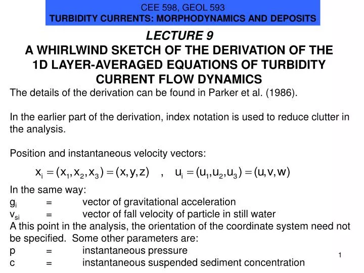
CEE 598, GEOL 593 TURBIDITY CURRENTS: MORPHODYNAMICS AND DEPOSITS. LECTURE 9 A WHIRLWIND SKETCH OF THE DERIVATION OF THE 1D LAYER-AVERAGED EQUATIONS OF TURBIDITY CURRENT FLOW DYNAMICS. The details of the derivation can be found in Parker et al. (1986).

E N D
CEE 598, GEOL 593 TURBIDITY CURRENTS: MORPHODYNAMICS AND DEPOSITS LECTURE 9 A WHIRLWIND SKETCH OF THE DERIVATION OF THE 1D LAYER-AVERAGED EQUATIONS OF TURBIDITY CURRENT FLOW DYNAMICS The details of the derivation can be found in Parker et al. (1986). In the earlier part of the derivation, index notation is used to reduce clutter in the analysis. Position and instantaneous velocity vectors: In the same way: gi = vector of gravitational acceleration vsi = vector of fall velocity of particle in still water A this point in the analysis, the orientation of the coordinate system need not be specified. Some other parameters are: p = instantaneous pressure c = instantaneous suspended sediment concentration
GOVERNING EQUATIONS OF THE INSTANTANEOUS FLOW The governing equations of the instantaneous flow are: The Navier-Stokes equations for momentum balance of the flow: the continuity equation for conservation of flow water mass: and the equation of conservation of suspended sediment mass: where usi denotes the velocity vector of a sediment particle, and as before
GOVERNING EQUATIONS OF THE INSTANTANEOUS FLOW contd. The Navier-Stokes equations for momentum balance can be rewritten as where v,ij denotes the viscous stress tensor, given as In addition, it is assumed here that the instantaneous sediment particle velocity usi is equal to the sum of the fluid velocity and the fall velocity: so that the equation of balance of suspended sediment becomes
THE AMBIENT WATER ABOVE THE CURRENT The ambient water above the turbidity current is assumed to be in hydrostatic balance with density a, so that the Navier-Stokes equation reduces to where pa denotes the ambient pressure.
THE BOUSSINESQ APPROXIMATION The turbidity current can induce some deviatoric pressure pd that varies about the ambient hydrostatic value: Now using the above relation and the relation of the previous slide to reduce the Navier-Stokes equation of two slides before, it is found that since f - a = aRc, The heart of the Boussinesq approximation is that the effect of the density difference between the bottom underflow and the ambient water (in this care created by the presence of sediment and so = Rc) is neglected in the acceleration terms (where Rc is small compared to 1) but kept in the gravity term (where it is all that is available to drive the flow):
THE REDUCED INSTANTANEOUS EQUATIONS where and
MEAN AND FLUCTUATING QUANTITIES FOR TURBULENT FLOW Turbidity currents need not be turbulent. (“Turbid” comes from a Latin root meaning “muddy”.) For example, laminar turbidity currents carrying mud can travel long distances before the mud settles out. In the absence of turbulence, however, any sediment that settles cannot be re-entrained into the flow. This means that most interesting cases involve turbulent flow. In the case of turbulent flow, the instantaneous parameters ui, c and p fluctuate about mean values. Here the mean values are denoted with an overbar, and the fluctuating values are denoted with a prime superscript: • Some rules of averaging are stated below • The average of the sum = the sum of the average. • A quantity that is already averaged cannot be averaged more. • Differentiation and averaging commute. • The average of the produce does not = the product of the average. • Thus if A and B are instantaneous parameters, e.g.
REYNOLDS-AVERAGED BALANCE EQUATIONS Averaging the balance equations over turbulence results in the forms where R,ij denotes the Reynolds stress due to turbulence, and FR,i denotes the Reynolds flux of suspended sediment: These terms quantify the tendency of turbulence to mix momentum and sediment mass, respectively, at rates that far exceed molecular processes. With this in mind, the viscous stress term in the momentum equation is neglected in subsequent slides.
2D FLOW OVER A BED We now use the geometry assumed earlier in the lecture. That is, x is a boundary-attached streamwise coordinate, z is a boundary-attached upward-normal coordinate, S <<1, gi and vsi are approximated as where vs is the scalar particle fall velocity (positive for vertical downward). In addition, the flow is assumed to be uniform in the y direction, with
SLENDER FLOW (BOUNDARY LAYER) APPROXIMATIONS For most cases of interest it can be assumed that , so that the equation of balance of suspended sediment mass reduces to According to the slender flow approximation, the characteristic distance Lc over which the flow changes in the streamwise (x) direction is taken to be large compared to the characteristic distance c (estimate of boundary layer thickness) over which flow changes in the upward normal (z) direction, so that In addition, it is assumed that a characteristic time for the flow to change Tc is at least as large as Lc/Uc, where Uc is a characteristic velocity of the flow.
BALANCE EQUATIONS APPROXIMATED FOR SLENDER FLOW The details of the application of the slender flow approximations are not shown here. They can be found in most books on turbulent flow. The reduced forms are where and F are now shorthand for R,xz and FR,z, respectively.
THE DEVIATORIC PRESSURE TERM Note that the upward normal momentum equation has reduced to a hydrostatic balance between the deviatoric pressure and the excess gravitational force due to sediment in the flow: Now high above the flow, the pressure distribution is ambient, so that Integrating the first equation using the second equation as a boundary condition, it is found that The streamwise momentum equation thus reduces to
LAYER INTEGRATION The streamwise momentum equation can be further rewritten with the aid of continuity, to the form: This equation is now integrated from z = 0 to z = (i.e. far above the current, where the ambient water is in hydrostatic balance) under the boundary conditions to yield where b is the bed shear stress, given as
LAYER INTEGRATION contd. The equation of continuity integrates under the boundary conditions of the previous slide and the further condition to yield: Note that the upward normal velocity is not taken to be zero at z = . This is a consequence of the boundary layer approximations. More specifically, we represents an entrainment velocity at which ambient flow is sucked into the flow across the interface. In the case of a steady flow, it acts to increase the forward flow discharge per unit width of the flow in the downstream direction.
LAYER INTEGRATION contd. The equation of balance of suspended sediment integrates with the aid of the previously-stated boundary conditions and the further boundary condition to: where Note that Fb denotes the upward normal flux of suspended sediment at the bed, or in other words the entrainment rate of sediment from the bed. Defining a dimensionless entrainment rate Es such that the balance equation for suspended sediment reduces to
THE TOP HAT APPROXIMATION We now drop the overbars in the equations, it now being understood that the quantities in question have been averaged over turbulence: For a first look at the form of the equations, we evaluate the integrals using the top hat approximations:
EQUATIONS IN “SHALLOW WATER” FORM Performing the integrations with the top hat approximations and adding the closure relations the resulting forms are found to be: Relations for ew, ro and Es were presented earlier in the lecture.
REDUCTION TO “BACKWATER FORMS” FOR STEADY FLOW DEVELOPING IN THE STREAMWISE DIRECTION For the case of steady flow, the equations to the right reduce to the forms below: where: Note that qs is the volume transport rate per unit width of suspended sediment.
CORRESPONDING “BACKWATER FORMS” FOR A RIVER For the case of steady flow, the equations to the right reduce to the forms below: where qs and qse retain their meanings from the previous slide, qw denotes the (constant) water discharge per unit width, and
CASE OF A CONSERVATIVE UNDERFLOW DRIVEN BY E.G. SALINE OR TEMPERATURE-MEDIATED BUOYANCY EFFECTS This case is obtained in the limit as vs 0. Here RC Fe, where Fe now denotes the layer-averaged fractional buoyancy excess of the bottom flow induced by salt or cold temperature. The equations reduce to the forms to the right. For a steady flow, they further reduce to the forms on the left. Note that the volume discharge qe of the fractional density excess per unit width is constant, hence the terminology “conservative”. The bulk Richardson number is now
“NORMAL” FLOW FOR A RIVER Consider the case of flow over a constant slope S. We further assume that the bed friction coefficient Cf is constant. In the case of a river, the equations reduce to: The equations admit a solution for a “normal” velocity Un and a “normal” depth Hn that are both constants. The governing equations for this solution are Using e.g. the Garcia-Parker sediment entrainment relation, the “normal” concentration Cn of suspended sediment is then given as
“NORMAL” FLOW FOR CONSERVATIVE DENSITY UNDERFLOW We again consider the case of a constant bed slope S and bed friction coefficient Cf. In the case of a conservative density underflow, the equation for U two slides back has a constant “normal” solution Un. This can be obtained by setting the numerator of the equation for dU/dx to 0, so that where the subscript “n” denotes the “normal values”. Using, for example the relation below for ewn the first equation can be solved iteratively for a constant normal Richardson number Rin. Once the (constant) transport rate per unit width of density excess qe = UHFe is specified, the normal flow velocity Un can be computed from the relation
SAMPLE SOLUTIONS FOR NORMAL FLOW OF A CONSERVATIVE DENSE UNDERFLOW
“NORMAL” FLOW FOR CONSERVATIVE DENSITY UNDERFLOW contd. The equation for dH/dx, i.e. reduces with the relation for normal Richardson number and the condition of constant qe = UHFe to give Thus for the normal solution, current thickness increases linearly (as it entrains ambient water), and fractional excess density decreases hyperbolically (as the ambient water dilutes the salt or heat deficiency in the current).
NO “NORMAL” FLOW SOLUTION EXISTS FOR A TURBIDITY CURRENT THAT FREELY EXCHANGES SEDIMENT WITH THE BED If there were a corresponding “normal” solution for a turbidity current, it would take the form where Un and qsn are constants However, if Un is given constant, then Es is also a constant Esn, where would also be constant. The equation for conservation of suspended sediment for a steady would then take the form so that qs could not be constan after all. That is, dilution of the flow due to the entrainment of ambient water acts to push the flow out of equilibrium.
CAN WE DO BETTER THAN THE TOPHAT APPROXIMATION? If we had some data, we might be able to determine some approximate similarity forms for u and c: Applying the constraints it follows that fu and fc must be such that For example, the top hat assumptions satisfy these constraints.
EXAMPLE BASED ON EXPERIMENTAL DATA The data and functions are from Parker et al. (1987). They can’t be said to be universal for any turbidity current, but they can help get a picture of the sructure of turbidity currents. ’ ’ fu fc
SHAPE FACTORS Consider the previously-introduced layer-integrated forms: Now substituting the similarity forms, and using previously-introduced closure forms for b, we and cb, we find the relations on the next slide.
SHAPE FACTORS contd. The integral forms now reduce to where 1, and 2 are order-one shape factors given by the relations The data of Parker et al. (1987) suggest values of 1 and 2 close to 0.99 and 1.00, respectively. Parker et al. (1986) called the above three conservation equations the “three-equation model”.
DENSITY STRATIFICATION EFFECTS In a turbidity current, the flow higher up can be expected to have a lower concentration, and thus a lower density, than the flow lower down. Such a flow is called stably stratified. As turbulence mixes in the vertical in a stably straified flow, it must lift heavy water up and light water down. The extra work required to do this acts to damp the turbulence Parker et al. (1986) developed a fairly simple layer-integrated model that accounts for density stratification. It is called the four-equation model. The additional equation governs the conservation of the kinetic energy of the turbulence.
KINETIC ENERGY OF THE TURBULENCE In addition to U, H and C, the four-equation model introduces a fourth variable, i.e. the layer-averaged kinetic energy of the turbulence per unit fluid mass. That is, The balance equation for turbulent kinetic energy takes the form where the shear velocity u is given as The term o denotes the rate of dissipation of the energy of the turbulence per unit mass due to viscosity.
PHYSICAL MEANING OF THE TERMS IN THE BALANCE EQUATION FOR THE KINETIC ENERGY OF THE TURBULENCE A full derivation of the equation for K is given in Parker et al. (1987). The terms are interpreted below. • a) b) c) d) e) f) g) h) • time rate of change of layer-integrated turbulent kinetic energy (TKE) • streamwise variation in the discharge per unit width of TKE • rate of production of TKE associated with bed shear • rate of production of TKE associated with the interface • rate of dissipation of TKE due to viscosity • rate at which TKE is consumed in holding the sediment in suspension • rate at which TKE is consumed in lifting the suspended sediment as water entrainment thickens the current • rate at which TKE is lost (gained) as new sediment is entrained upward from (deposited downward onto) the bed • Terms f), g) and (in a flow that entrains sediment in the net) h) act to damp turbulence due to the presence of sediment.
CLOSURE ASSUMPTIONS IN THE FOUR-EQUATION MODEL In the four-equation model, the boundary shear stress is related to K rather than U: . Here the coefficient is estimated as 0.1. Note that this means the sediment entrainment rate Es now also depends on K rather than U: so that if K is damped then Es is throttled as well. The parameter o is given as where cD is an “equivalent” friction coefficient.
THE FULL FOUR-EQUATION MODEL The governing equations are where ew is a specified function of Ri as before, Es is a function of K as outlined in the previous slide, and the form for o is specified in the previous slide.
“BACKWATER FORMS” FOR STEADY FLOW DEVELOPING IN THE STREAMWISE DIRECTION: THE CASE OF THE FOUR-EQUATION MODEL
REFERENCES Garcia, M, and G. Parker, 1991, Entrainment of bed sediment into suspension. Journal of Hydraulic Engineering, 117(4), 414‑435. Parker, G., 1982, Conditions for the ignition of catastrophically erosive turbidity currents. Marine Geology, 46, pp. 307‑327, 1982. Parker, G., Y. Fukushima, and H. M. Pantin, 1986, Self‑accelerating turbidity currents. Journal of Fluid Mechanics, 171, 45‑181. Parker, G., M. H. Garcia, Y. Fukushima, and W. Yu, 1987, Experiments on turbidity currents over an erodible bed., Journal of Hydraulic Research, 25(1), 123‑147.