Download
1 / 54
540 likes | 686 Views
CPS 196.03: Information Management and Mining Association Rules and Frequent Itemsets. Apriori Algorithm. Method: Let k=1 Generate frequent itemsets of length 1 Repeat until no new frequent itemsets are identified Generate length (k+1) candidate itemsets from length k frequent itemsets

E N D
CPS 196.03: Information Management and Mining Association Rules and Frequent Itemsets
Apriori Algorithm • Method: • Let k=1 • Generate frequent itemsets of length 1 • Repeat until no new frequent itemsets are identified • Generate length (k+1) candidate itemsets from length k frequent itemsets • Prune candidate itemsets containing subsets of length k that are infrequent • Count the support of each candidate by scanning the DB • Eliminate candidates that are infrequent, leaving only those that are frequent
Generating Candidate ItemSets • Exhaustive enumeration • F(k-1) x F(1) • Using (lexicographic) ordering • F(k-1) x F(k-1) • Will hashing help?
Reducing Number of Comparisons • Candidate counting: • Scan the database of transactions to determine the support of each candidate itemset • To reduce the number of comparisons, store the candidates in a hash structure • Instead of matching each transaction against every candidate, match it against candidates contained in the hashed buckets
Generate Hash Tree Hash function 3,6,9 1,4,7 2,5,8 • Suppose you have 15 candidate itemsets of length 3: • {1 4 5}, {1 2 4}, {4 5 7}, {1 2 5}, {4 5 8}, {1 5 9}, {1 3 6}, {2 3 4}, {5 6 7}, {3 4 5}, {3 5 6}, {3 5 7}, {6 8 9}, {3 6 7}, {3 6 8} • You need: • Hash function • Max leaf size: max number of itemsets stored in a leaf node (if number of candidate itemsets exceeds max leaf size, split the node)
2 3 4 1 2 5 4 5 7 1 2 4 5 6 7 6 8 9 3 5 7 4 5 8 3 6 8 3 6 7 3 4 5 1 3 6 14 5 1 5 9 3 5 6 Association Rule Discovery: Hash tree Hash Function Candidate Hash Tree 1,4,7 3,6,9 2,5,8 Hash on 1, 4 or 7
2 3 4 1 25 4 5 7 1 2 4 5 6 7 6 8 9 3 5 7 4 58 3 6 8 3 6 7 3 4 5 1 3 6 1 4 5 1 5 9 3 5 6 Association Rule Discovery: Hash tree Hash Function Candidate Hash Tree 1,4,7 3,6,9 2,5,8 Hash on 2, 5 or 8
2 3 4 1 2 5 4 5 7 1 2 4 5 6 7 6 8 9 3 5 7 4 5 8 36 8 36 7 3 4 5 1 3 6 1 4 5 1 5 9 3 5 6 Association Rule Discovery: Hash tree Hash Function Candidate Hash Tree 1,4,7 3,6,9 2,5,8 Hash on 3, 6 or 9
Subset Operation Given a transaction t, what are the possible subsets of size 3?
Hash Function 3 + 2 + 1 + 5 6 3 5 6 1 2 3 5 6 2 3 5 6 1,4,7 3,6,9 2,5,8 1 4 5 1 3 6 3 4 5 4 5 8 1 2 4 2 3 4 3 6 8 3 6 7 1 2 5 6 8 9 3 5 7 3 5 6 5 6 7 4 5 7 1 5 9 Subset Operation Using Hash Tree transaction
Hash Function 2 + 1 + 1 5 + 3 + 1 3 + 1 2 + 6 5 6 5 6 1 2 3 5 6 3 5 6 3 5 6 2 3 5 6 1,4,7 3,6,9 2,5,8 1 4 5 4 5 8 1 2 4 2 3 4 3 6 8 3 6 7 1 2 5 3 5 6 3 5 7 6 8 9 5 6 7 4 5 7 Subset Operation Using Hash Tree transaction 1 3 6 3 4 5 1 5 9
Hash Function 2 + 1 5 + 1 + 3 + 1 3 + 1 2 + 6 3 5 6 5 6 5 6 1 2 3 5 6 2 3 5 6 3 5 6 1,4,7 3,6,9 2,5,8 1 4 5 4 5 8 1 2 4 2 3 4 3 6 8 3 6 7 1 2 5 3 5 7 3 5 6 6 8 9 4 5 7 5 6 7 Subset Operation Using Hash Tree transaction 1 3 6 3 4 5 1 5 9 Match transaction against 11 out of 15 candidates
Factors Affecting Performance • Choice of minimum support threshold • lowering support threshold results in more frequent itemsets • this may increase number of candidates and max length of frequent itemsets • Dimensionality (number of items) of the data set • more space is needed to store support count of each item • if number of frequent items also increases, both computation and I/O costs may also increase • Size of database • since Apriori makes multiple passes, run time of algorithm may increase with number of transactions • Average transaction width • number of subsets in a transaction increases with its width • this may increase max length of frequent itemsets and traversals of hash tree
Compact Representation of Frequent Itemsets • Some itemsets are redundant because they have identical support as their supersets • Number of frequent itemsets • Need a compact representation
Compression of Itemset Information Transaction Ids Not supported by any transactions
Maximal Frequent Itemset An itemset is maximal frequent if none of its immediate supersets is frequent Maximal Itemsets Infrequent Itemsets Border
Closed Itemset • An itemset is closed if none of its immediate supersets has the same support as the itemset
Maximal vs Closed Itemsets Transaction Ids Not supported by any transactions
Maximal vs Closed Frequent Itemsets Closed but not maximal Minimum support = 2 Closed and maximal # Closed = 9 # Maximal = 4
Why Do We Care About Closed Itemsets? • Compact representation of frequent itemsets • Helps if there are many frequent itemsets • There are efficient algorithms that can efficiently find the closed itemsets (and only them) • HW Exercise: Come up with an algorithm to generate all info about frequent itemsets given info about closed frequent itemsets? • Closed itemsets help identify redundant association rules • E.g., if {b} and {b,c} have the same support: then would you care about {b} -> {d} or {b,c} -> {d}?
Toivonen’s Algorithm --- (1) • Start as in the simple algorithm, but lower the threshold slightly for the sample. • Example: if the sample is 1% of the baskets, use s/125 as the support threshold rather than s /100. • Goal is to avoid missing any itemset that is frequent in the full set of baskets.
Toivonen’s Algorithm --- (2) • Add to the itemsets that are frequent in the sample the negative border of these itemsets. • An itemset is in the negative border if it is not deemed frequent in the sample, but all its immediate subsets are.
Example • ABCD is in the negative border if and only if it is not frequent, but all of ABC, BCD, ACD, and ABD are.
Toivonen’s Algorithm --- (3) • In a second pass, count all candidate frequent itemsets from the first pass, and also count the negative border. • If no itemset from the negative border turns out to be frequent, then the candidates found to be frequent in the whole data are exactly the frequent itemsets.
Toivonen’s Algorithm --- (4) • What if we find something in the negative border is actually frequent? • We must start over again! • Try to choose the support threshold so the probability of failure is low, while the number of itemsets checked on the second pass fits in main-memory.
Alternative Methods for Frequent Itemset Generation • Traversal of Itemset Lattice • General-to-specific vs Specific-to-general
Alternative Methods for Frequent Itemset Generation • Traversal of Itemset Lattice • Equivalent Classes
Alternative Methods for Frequent Itemset Generation • Traversal of Itemset Lattice • Breadth-first vs Depth-first
Alternative Methods for Frequent Itemset Generation • Representation of Database • horizontal vs vertical data layout
ECLAT • For each item, store a list of transaction ids (tids) TID-list
ECLAT • Determine support of any k-itemset by intersecting tid-lists of two of its (k-1) subsets. • 3 traversal approaches: • top-down, bottom-up and hybrid • Advantage: very fast support counting • Disadvantage: intermediate tid-lists may become too large for memory
Bottleneck of Frequent-pattern Mining • Multiple database scans are costly • Mining long patterns needs many passes of scanning and generates lots of candidates • To find frequent itemset i1i2…i100 • # of scans: 100 • # of Candidates: (1001) + (1002) + … + (110000) = 2100-1 = 1.27*1030 ! • Bottleneck: candidate-generation-and-test • Can we avoid candidate generation?
FP-growth Algorithm • Use a compressed representation of the database using an FP-tree • Once an FP-tree has been constructed, it uses a recursive divide-and-conquer approach to mine the frequent itemsets
FP-tree construction null After reading TID=1: A:1 B:1 After reading TID=2: null B:1 A:1 B:1 C:1 D:1
FP-Tree Construction Transaction Database null B:3 A:7 B:5 C:3 C:1 D:1 Header table D:1 C:3 E:1 D:1 E:1 D:1 E:1 D:1 Pointers are used to assist frequent itemset generation
{} Header Table Item frequency head f 4 c 4 a 3 b 3 m 3 p 3 f:4 c:1 c:3 b:1 b:1 a:3 p:1 m:2 b:1 p:2 m:1 Construct FP-tree from Transaction Database TID Items bought (ordered) frequent items 100 {f, a, c, d, g, i, m, p}{f, c, a, m, p} 200 {a, b, c, f, l, m, o}{f, c, a, b, m} 300 {b, f, h, j, o, w}{f, b} 400 {b, c, k, s, p}{c, b, p} 500{a, f, c, e, l, p, m, n}{f, c, a, m, p} min_support = 3 • Scan DB once, find frequent 1-itemset (single item pattern) • Sort frequent items in frequency descending order, f-list • Scan DB again, construct FP-tree F-list=f-c-a-b-m-p
Benefits of the FP-tree Structure • Completeness • Preserve complete information for frequent pattern mining • Never break a long pattern of any transaction • Compactness • Reduce irrelevant info—infrequent items are gone • Items in frequency descending order: the more frequently occurring, the more likely to be shared • Never be larger than the original database (not count node-links and the count field)
Partition Patterns and Databases • Frequent patterns can be partitioned into subsets according to f-list • F-list=f-c-a-b-m-p • Patterns containing p • Patterns having m but no p • … • Patterns having c but no a nor b, m, p • Pattern f • Completeness and non-redundancy
{} Header Table Item frequency head f 4 c 4 a 3 b 3 m 3 p 3 f:4 c:1 c:3 b:1 b:1 a:3 p:1 m:2 b:1 p:2 m:1 Find Patterns From P-conditional Database • Starting at the frequent item header table in the FP-tree • Traverse the FP-tree by following the link of each frequent item p • Accumulate all of transformed prefix paths of item p to form p’s conditional pattern base Conditional pattern bases item cond. pattern base c f:3 a fc:3 b fca:1, f:1, c:1 m fca:2, fcab:1 p fcam:2, cb:1
{} f:3 c:3 a:3 m-conditional FP-tree From Conditional Pattern-bases to Conditional FP-trees • For each pattern-base • Accumulate the count for each item in the base • Construct the FP-tree for the frequent items of the pattern base • m-conditional pattern base: • fca:2, fcab:1 {} Header Table Item frequency head f 4 c 4 a 3 b 3 m 3 p 3 All frequent patterns relate to m m, fm, cm, am, fcm, fam, cam, fcam f:4 c:1 c:3 b:1 b:1 a:3 p:1 m:2 b:1 p:2 m:1
{} f:3 c:3 am-conditional FP-tree {} f:3 c:3 a:3 m-conditional FP-tree Recursion: Mining Each Conditional FP-tree Cond. pattern base of “am”: (fc:3) {} Cond. pattern base of “cm”: (f:3) f:3 cm-conditional FP-tree {} Cond. pattern base of “cam”: (f:3) f:3 cam-conditional FP-tree
Mining Frequent Patterns With FP-trees • Idea: Frequent pattern growth • Recursively grow frequent patterns by pattern and database partition • Method • For each frequent item, construct its conditional pattern-base, and then its conditional FP-tree • Repeat the process on each newly created conditional FP-tree • Until the resulting FP-tree is empty, or it contains only one path—single path will generate all the combinations of its sub-paths, each of which is a frequent pattern
Rule Generation • Given a frequent itemset L, find all non-empty subsets f L such that f L – f satisfies the minimum confidence requirement • If {A,B,C,D} is a frequent itemset, candidate rules: ABC D, ABD C, ACD B, BCD A, A BCD, B ACD, C ABD, D ABCAB CD, AC BD, AD BC, BC AD, BD AC, CD AB, • If |L| = k, then there are 2k – 2 candidate association rules (ignoring L and L)
Rule Generation • How to efficiently generate rules from frequent itemsets? • In general, confidence does not have an anti-monotone property c(ABC D) can be larger or smaller than c(AB D) • But confidence of rules generated from the same itemset has an anti-monotone property • e.g., L = {A,B,C,D}: c(ABC D) c(AB CD) c(A BCD) • Confidence is anti-monotone w.r.t. number of items on the RHS of the rule
Pruned Rules Rule Generation for Apriori Algorithm Lattice of rules Low Confidence Rule
Pattern Evaluation • Association rule algorithms tend to produce too many rules • many of them are uninteresting or redundant • Redundant if {A,B,C} {D} and {A,B} {D} have same support & confidence • Interestingness measures can be used to prune/rank the derived patterns • In the original formulation of association rules, support & confidence are the only measures used
Interestingness Measures Application of Interestingness Measure
f11: support of X and Yf10: support of X and Yf01: support of X and Yf00: support of X and Y Computing Interestingness Measure • Given a rule X Y, information needed to compute rule interestingness can be obtained from a contingency table Contingency table for X Y Used to define various measures • support, confidence, lift, Gini, J-measure, etc.
Association Rule: Tea Coffee • Confidence= P(Coffee|Tea) = 0.75 • but P(Coffee) = 0.9 • Although confidence is high, rule is misleading • P(Coffee|Tea) = 0.9375 Drawback of Confidence