Download
1 / 29
290 likes | 407 Views
July 19, 2008 Martin Bobb Joseph Marmerstein Feibi Yuan Caden Ohlwiler. SI 2008: Study of Wave Motion. Introduction. Goal -- Model Motion of Waves MATLAB -- Programming Application Method Approximating the Wave Equation. MATLAB. Software with simulation and visualization functions

E N D
July 19, 2008 Martin Bobb Joseph Marmerstein Feibi Yuan Caden Ohlwiler SI 2008: Study of Wave Motion
Introduction • Goal -- Model Motion of Waves • MATLAB -- Programming Application • Method • Approximating the Wave Equation
MATLAB • Software with simulation and visualization functions • “Matrix Laboratory” • Uses matrices to perform complex calculations • Most of our group has limited programming experience • No previous MATLAB experience
Wave Equation • This is a partial differential equation (college level math) • Continuous • Approximated using the Finite Difference Method
Boundary Conditions • Behavior at the edges of the simulation • Fixed • Out of phase reflection • Free • In phase reflection • No-reflection boundaries are very difficult
Two Dimensional Waves • Wave in x-y plane • Like the surface of a lake • Third dimension represents wave height • Set conditions to represent air • Wave propagation speed • Viscosity • Nyquist frequency • Highest frequency that can be resolved accurately • Simulation must run at twice that • 22100 Hz
Initial Disturbances and Forcing Functions • Initial disturbance • One disturbance, dissipates over time (much like a shock wave) • Forcing Function • Continuous Output • Similar to a speaker playing a single note • Follows the path of a sine wave
Viscosity • Viscosity • Measure of the resistance to motion from a fluid • Adds a new term to wave equation • Makes the wave equation more realistic • Molasses vs. Water
Virtual Throat Simulation • Two walls, space in between • Three microphones • Behind, inside and in front of the throat • Forcing function • 20 Hz
Fast Fourier Transforms (FFTs) • Fourier Transform • Mathematical method • Takes a function in time and changes it to frequency components • Shows the frequencies at which a system is responding • Fast Fourier Transform • Numerical method • Computes the Fourier Transform quickly
FFT On Microphone #1 Relative Magnitude Frequency (Hz)
FFT on Microphone #2 Relative Magnitude Frequency (Hz)
FFT on Microphone #3 Relative Magnitude Frequency (Hz)
Virtual Room Simulation Based on geometry of BALE Gallery room Forcing Function of 110 Hz “A” string on a guitar Three microphones Behind column, in front of column, behind “speakers” Simulation was not entirely successful Solution tends to “ring”
Three Dimensional Waves • Volume divided into finite pieces • Wave “height” represents compression instead of actual wave height • Requires more computing power • Simulations take more time • Can take hours • Waves dissipate much faster than in 2D • Forcing functions have a less noticeable effect
Three Dimensional Visualization • Tried multiple techniques in MATLAB • Isosurfaces • Generates meshes at specific wave heights • Did not provide relevant visual • Volume Rendering • Passes light through the simulation • Used in 3D visualizations • Alpha mapping • Does not display wave heights close to zero • Makes them transparent • White space isn’t necessarily motionless
Conclusions • Learned about wave motion • Computer simulations are difficult to make exact • Everything is approximated • Learned how to program in MATLAB • Learned about simulation and visualization • Learned how to use Linux
Acknowledgments • Troy Baer -- Project Leader • Armen Ezekielian -- MATLAB support • Elaine Pritchard -- Food/snacks/organization • Daniel & Brianna -- Dorm supervisors • All the staff that gave presentations • James Rader -- Gallery blueprints • Third-party MATLAB add-ons: • Blinkdagger.com – positiveFFT function • Mathworks.com -- vol3d function