Download
1 / 32
320 likes | 422 Views
Robust Extraction of Vertices in Range Images by Constraining the Hough Transform. Dimitrios Katsoulas Institute for Pattern Recognition and Image Processing University of Freiburg. Introduction. Depalletizing : automatic unloading of piled objects via a robot .

E N D
Robust Extraction of Vertices in Range Images by Constraining the Hough Transform Dimitrios Katsoulas Institute for Pattern Recognition and Image Processing University of Freiburg
Introduction • Depalletizing: automatic unloading of piled objects via a robot. • How important is a solution to the problem? • Applications: Post, distribution centres, airports. • We deal with objects most frequently encountered: Boxes, box-like objects (e.g. sacks full of material)
Construction of an automatic system • Sensor: Range sensor for data acquisition, since it is of advantage to have depth information. • Modelling: geometric parametric models: superquadrics. • Recovery: Based on hypothesis generation and refinement. • [ChenKak89]: 3D Vertices provide the strongest constraints for generating hypotheses about object pose in space Vertex detection of extreme importance for hypothesis generation!!
Vertex detection in Images • Many approaches for detecting corners in intensity images, e.g. [Harris.et.al 88], [Smith.et.al 98] (SUSAN), [Deriche.et.al 92], [Zhang.et.al 94] • In range images: The majority employs region information e.g. [ChenKak 89], [Baerveldt 93]. • Problem: More than one surface needs to be exposed to the range sensor. • Our approach: Utilizes boundary information, based on Hough Transform: • Image acquisition • Linear boundary detection in 3D • Boundary grouping
ROADMAP • Data acquisition • Detection of linear object boundaries in 3D • Edge detection • Parameter recovery with the Hough Transform • Line Detection in 3D • Model Selection • Boundary grouping • Experiments • Discussion
ROADMAP • Data acquisition • Detection of linear object boundaries in 3D • Edgedetection • Parameter recovery with the Hough Transform • Line Detection in 3D • Model Selection • Boundary grouping • Experiments • Discussion
Edge map generation • We use the detector of [Jiang.et.al 00] which approximates the scan lines with linear and parabolic segments. • Advantage with regard to local edge detectors: Accuracy, ability to detect crease edges. • Problem: Error in localizing edge points, models do not perfectly express the objects.
Output of edge detection How can we detect linear boundaries from an edge map?
Parameter recovery with the Standard Hough Transform Line Equation:
Problems of the SHT • Localization error not addressed! • Computationally inefficient and memory consuming: • If N the dof of the model sought • p the number of parameters constrained by each point in the image space • Then mapping of each image point requires incrementing all bins comprising a N-p - dimensional manifold of the accumulator. • Test case 3D lines: N = 4, p = 2 4D accumulator, update of a 2D manifold per mapping.
TRIAL Improving the performance of Hough transform by problem decomposition • Idea: Decompose the transform into sub-problems: • Select set of points with cardinality d (d<N) • Consider r random subsets of the remaining points with cardinality v, so that d+ v= N • Map the union to the parameter space. • Perform t trials. • Find peaks. • Adjustment of d,r,t results to a variety of approaches: Most representative [Leavers 92] , [Olson 00], [Olson 01].
Recognition using Decomposition and Randomization [Olson 01] • Parameter selection: • d = N -1 • r = n -1, where n the number of edge points in image • If the user defined probability of failure in finding a model and m the minimum number of expected to lie on the model then:
Constraining the Hough Transform Line equation:
Advantages of RUDR • Complexity: O(tr) t: constant O(n) • By selecting d = N - 1: • The transform is constrained to lie on a 1D curve, the Hough Curve • 1D data structures are used for accumulation Memory requirements O(n) • Accurate error propagation in the parameter space.
Line detection in 3D • 3D case: points constrain two line parameters. • Thereby, we cannot constrain the transform to lie on a curve. • Solution: Break down the problem in two 2D sub-problems: • Determine 2 line parameters on the image (XZ) plane. • Determine the remaining on the plane defined by the detected line and the Y axis.
The problem of redundancy • Our algorithm does not guarantee that only one point of the same boundary is used as distinguished point. • Point removal is problematic. • Instead of retaining a locally sufficient model we: • Wait until all trials take place • Retain models satisfying global optimality criteria • Criteria: Favor models which describe bigger number of image points with higher accuracy. • Selection via MDL
Selecting the optimal lines • If M models recovered, we consider the matrix: and the binary vector • Diagonal elements: • Off- diagonals: • Benefit function: • Model recovery:
Selecting optimal lines (2) • Maximization though simulated annealing or neural networks computationally inefficient. • We adopt the greedy algorithm of proposed in [jaklic et al 00]
Complexity: since The Detection-Selection process
ROADMAP • Data acquisition • Detection of linear object boundaries in 3D • Edge detection • Parameter recovery with the Hough Transform • Line Detection in 3D • Model Selection • Boundary grouping • Experiments • Discussion
Boundary grouping • 3D vertex: Aggregate consisting of: • Two orthogonal 3D line segments. • Vertex point. • Ideally: If X,Y linear segments the dot product of their direction vectors should be zero: • Threshold: difficult to set, depends on the application and on the uncertainty in calculation of line parameters. • Can we avoid multiple thresholds? Yes by introducing statistical tests.
Statistical testing the geometric relation • We adopt the framework of [Foerstner 00] for its compactness and straightforwardness. • Dot product: Bilinear function of two stochastic vectors: • The variance of their dot product is given by:
Statistical testing the geometric relation (2) • The optimal test statistic for the hypothesis: is given by: • A significance value is selected. • If the hypothesis that the relation holds can be rejected. • Overall algorithm for boundary grouping: • Consider all pairs of lines. • The pairs passing the test along their intersection points are the detected vertices.
Discussion • System advantages: • Robustness: Error propagation, statistical test for grouping • Accuracy: Model selection. • Computational efficiency: Linear complexity to the number of edge points. • Low memory consumption: 1D accumulators used. • Versatility: Deals with both piled and neatly placed configurations. • Simplicity. • System drawbacks: What if the objects are placed very close one after another?