Download
1 / 21
220 likes | 301 Views
Simulation of flame acceleration and DDT in H2-air mixture with a flux limiter centred method Knut Vaagsaether, Vegeir Knudsen and Dag Bjerketvedt. Outline Introduction Models and numerics Physical experiments Numerical experiments Conclusion.

E N D
Simulation offlame acceleration and DDT in H2-air mixture with a flux limiter centred method Knut Vaagsaether, Vegeir Knudsen and Dag Bjerketvedt ICHS Pisa 2005
Outline • Introduction • Models and numerics • Physical experiments • Numerical experiments • Conclusion ICHS Pisa 2005
The goal of this work is to simulate the explosion process from a weak ignition source through flame acceleration and DDT to a detonation • The simulation tool is based on large eddy simulation (LES) of the filtered conservation equations with a 2. order centred TVD method • Numerical results are compared to experimental results with pressure records ICHS Pisa 2005
Filtered conservation equations of mass, momentum and energy ICHS Pisa 2005
Turbulence model, by Menon et.al. ICHS Pisa 2005
In addition to the mass, momentum, energy and k, two other variables are conserved • Two reaction variables, α and z • α is a variable for the production of radicals where no energy is released • z is a variable for the consumption of radicals (exothermal reactions) ICHS Pisa 2005
α is only solved for the unreacted gas • α keeps track of the induction time • If α is below 1, no exothermal reaction is taking place • If α reaches 1 an exothermal reaction occurs • The production term of α is an Arrhenius function and can be assumed to be 1/τ ICHS Pisa 2005
The exothermal reactions are handeled in two ways • If the flame is a deflagration wave, a Riemann solver is used to calculate the states at each side of the flame • The Riemann solver use the burning velocity as the reaction rate • If the flame is a detonation wave or α reaches 1, another reaction model is used, presented by Korobeinikov (1972) ICHS Pisa 2005
Burning velocity as a function of velocity fluctuations, presented by Flohr and Pitsch (2000) • This model is developed for lean premixed combustion in gas turbine combustors ICHS Pisa 2005
Flame tracking with the G-equation • Where vf is the local particle velocity in front of the flame • G is negative in the unburned gas • The G0 surface is set to be immediately in front of the flame ICHS Pisa 2005
Solvers • A flux limiter centered method (FLIC) to solve the hyperbolic part of the equations, an explicit 2nd order TVD method • Central differencing for the diffusion terms • Godunov splitting for dimensions, diffusion terms and sub-models • 4. order RK for ODEs ICHS Pisa 2005
Experimental setup • 30% hydrogen in air • 1 atm, 20°C • Closed tube • 10.7 cm ID • Spark plug ignition at p0 • 0.5 m between sensors • 1.5 between p0 and p1 • 3 cm orifice in obstacle ICHS Pisa 2005
Experimental results, pressure records ICHS Pisa 2005
Numerical setup • Same conditions as physical experiments • Assume cylindrical coordinates • 2D • Axis-symmetric • Carthesian, homogeneous grid • CV length 2 mm (~50 000 CV) • CFL number 0.9 ICHS Pisa 2005
Comparison of pressure history at sensor p0 ICHS Pisa 2005
Comparison of pressure history at p2 ICHS Pisa 2005
Density in a 240 mm X 107 mm area • Time difference is 0.025 ms • DDT occurs between image 1 and 2 ICHS Pisa 2005
Mach numberat center line behind the obstacle as the flame reaches the opening ICHS Pisa 2005
Discussion and conclusion • The pressure in the ignition end of the tube is simulated with some accuracy, even with these assumtions • The detonation wave is simulated very accurate compared to the experiments which means that the Korobeinikov model is good enough for this work • A DDT is simulated ICHS Pisa 2005
Discussion and conclusion • Some discrepancies between numerical and physical results in the ignition part (deflagration) • 2D • Boundary conditions for the G-equation • Burning velocity model • The DDT is simulated too late • 2D • Induction time • Errors in pressure from the ignition part • Is it possible with LES? ICHS Pisa 2005
Further work • 3D simulation should be performed • Boundary conditions for the G-equation? • Burning velocity model • Adaptive mesh refinement • A new model for the induction time ICHS Pisa 2005