Download
1 / 16
160 likes | 305 Views
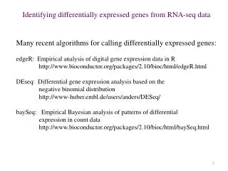
Identifying differentially expressed genes from RNA- seq data. Many recent algorithms for calling differentially expressed genes: edgeR : Empirical analysis of digital gene expression data in R http:// www.bioconductor.org /packages/2.10/ bioc /html/ edgeR.html

E N D
Identifying differentially expressed genes from RNA-seq data Many recent algorithms for calling differentially expressed genes: edgeR: Empirical analysis of digital gene expression data in R http://www.bioconductor.org/packages/2.10/bioc/html/edgeR.html DEseq: Differential gene expression analysis based on the negative binomial distribution http://www-huber.embl.de/users/anders/DESeq/ baySeq: Empirical Bayesian analysis of patterns of differential expression in count data http://www.bioconductor.org/packages/2.10/bioc/html/baySeq.html
Identifying differentially expressed genes from RNA-seq data Why can’t we use the same software for microarray data analysis? • 1. Microarray data are continuous values. Sequence data are discrete values of • read counts. • e.g. 5.342 signal intensity versus 5 counts • Reproducibility of RNA-seq measurements is different for low-abundance versus • high-abundance transcripts – this is called over-dispersion
Overdispersion: variance of replicates is higher for high-abundance reads
baySeq Empirical Bayesian analysis of patterns of differential expression in count data http://www.bioconductor.org/packages/2.10/bioc/html/baySeq.html Identifies differentially expressed genes between 2 or more samples using replicated RNA-seq data
Bayes’ Theorem P (M | D) = P (D | M) * P (M) P (D) Read in English: The Probability that your Model is correct Given ( | ) the Data is equal to the Probability of your Data Given the Model times the Probability of your Model divided by the Probability of the Data What the hell does this mean?
Bayes’ Theorem: wikipedia’s ridiculous example Your friend had a conversation with someone who happened to have long hair. What is the probability that that person was a woman, given that you know ~50% of people are women and ~75% of women have long hair. P (W) = Probability that this person was a woman = 0.5 P (L | W) = Probability that the person had long hair IF the person is a woman = 0.75 P (L | M) = Probability that the person had long hair IF that person is a man = 0.3 P (L) = Probability that any random person has long hair = P (L | W) * P (W) = 75% of 50% of the population = 0.75*0.5 = 0.375 + P (L | M) * P (M) = 30% of 50% of the population = 0.3 * 0.5 = 0.15 So: P (W|L) = P(L|W)*P(W) = P(L|W)*P(W) = 0.714 P(L) P (L|W)*P(W) + P (L|M)*P(M)
Bayes’ Theorem P (M | D) = P (D | M) * P (M) P (D) Read in English: The Probability that your Model is correct Given ( | ) the Data is equal to the Probability of your Data Given the Model times the Probability of your Model divided by the Probability of the Data P is called the ‘Posterior Probability’ that this Model is the right one to describe your data. Each gene will have a PP for each model, where S PP = 1. The Bigger the PP, the more likely this is the right model. Posterior Probability is NOT a p-value!
Bayes’ Theorem Imagine you have three RNA-seq replicates of two samples (WT vs mutant). There are two models for each gene M0 = the model that your gene is NOT differentially expressed across the 2 samples MDE = the model that a given gene IS differentially expressed P (M0 | DgeneX) = P (DgeneX | M0) * P (M0) P (DgeneX) P (MDE | DgeneX) = P (DgeneX | MDE) * P (MDE) P (DgeneX) We don’t know some of these factors ( e.g. P(D|M) ), but we can describe the data with some parameter set called q (which includes mean and stdev of count data across replicates of each gene)
How to model the mean and standard deviation of your replicates: Poisson Distribution: Accounts for random fluctuations wikepedia E.g. Infecting a cell culture with viral particles. l = Multiplicity of Infection (MOI) = # of viral particles/cell in your culture
Overdispersion: variance of replicates is higher for high-abundance reads
How to model the mean and standard deviation of your replicates: Negative Binomial Distribution: Mean and variance are different Notice the wider spread on the right side of each distribution, for higher numbers
baySeq Empirical Bayesian analysis of patterns of differential expression in count data http://www.bioconductor.org/packages/2.10/bioc/html/baySeq.html Imagine you have triplicate measurements of sample A and sample B. We want to identify genes differentially expressed (DE) in A versus B. Arep1 Arep2 Brep1 Brep2 tuple: simply S counts per transcription unit We define TWO possible models: NO DE (NDE): Arep1= Arep2= Brep1= Brep2 we say that the data for all samples was drawn from the same distribution (* i.e. same mean and standard deviation, if normally distributed) DE: Arep1 = Arep2NOT EQUAL Brep1 = Brep2 A and B replicates are drawn from two different distributions
baySeq Empirical Bayesian analysis of patterns of differential expression in count data http://www.bioconductor.org/packages/2.10/bioc/html/baySeq.html Next, we use Bayes’ Rule to try to estimate the probability that the DE model is true for geneX prior probability P (MDE | DgeneX) = P(DgeneX|MDE) * P(MDE) P(DgeneX) baySeq tries to use data sharing across the dataset to estimate the components on the right side of the equation P (DgeneX|MDE) = Int[ P(DgeneX| K, MDE) * P(K | MDE) ]dK where K is the parameter set of q (mean, dispersion) for each gene in each replicate ** q for each gene is estimated by looking at all data in the replicates
baySeq Empirical Bayesian analysis of patterns of differential expression in count data http://www.bioconductor.org/packages/2.10/bioc/html/baySeq.html prior probability P (MDE | DgeneX) = P(DgeneX|MDE) * P(MDE) P(DgeneX) The prior probability is the probability of M before any data are considered. Here: 1. Guess at a starting prior probability for MDE 2. Iteratively test different alternatives 3. Repeat until ‘convergence’ (P(MDE) does not change with more iterations) * For data with strong DE signal, the posterior probability is not very dependent on the starting prior probability P(MDE)