Statistical tools applied to the H I Magellanic Bridge

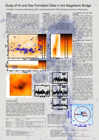
1. Statistical tools applied to the HI Magellanic Bridge Erik Muller (UOW, ATNF) Supervisors: Lister Staveley-Smith (ATNF) Bill Zealey (UOW) Statistical Tools applied to the Magellanic Bridge

2. Introduction • Statistical tools provide a means to • compare populations of similar objects between different systems • Understand and model general trends and behaviours. • Distinguish between sub-populations • Spectral correlation function (SCF): Measures spectral similarity as a function of radial separation • Power spectrum analysis (PS): Measures power as a function of scale, and as a function of velocity range. • Both SCF and PS have been used to infer information about the third spatial dimension. Statistical Tools applied to the Magellanic Bridge

3. Data set (ATCA +Parkes): Peak pixel HI map, Magellanic Bridge Statistical Tools applied to the Magellanic Bridge

4. Spectral Tools 1: • Specral Correlation function: • Compares two spectra separated by Δr, and makes an estimate of their ‘similarity’ • A 2D map of mean SCF shows rate of change (or degree of corrleation) of SCF with Δr and θ • Has been used to confirm a characteristic length for the scale height of the LMC, by measuring the radius of decorrelation (Padoan et al. 2001) • In this case, SCF shows that MB spectra has a longer decorrelation length in the east-west direction. (Tidal stretching) Statistical Tools applied to the Magellanic Bridge

5. Spectral Tools 2: • Spatial power spectrum • Used to show the range of spatial scales present in source • Highlights any process favouring a particular scale. (Eg. Elmegreen, Kim, Staveley-Smith, 2001) • Using velocity averaging, is can be used to show the relative contributions of density and velocity dominated fluctuations. (Lazarian & Pogosyan, 2001) Statistical Tools applied to the Magellanic Bridge

6. Δr Δr Δr Spectral Correlation functionHow it works: Statistical Tools applied to the Magellanic Bridge

7. SCF output maps: Statistical Tools applied to the Magellanic Bridge

8. T maps 55 pixels 37 pixels SCF maps Statistical Tools applied to the Magellanic Bridge

9. Fits in E-W and N-S directions (central 5 rows/columns) ΣT=1.0x106 K.km/s ΣT=7.5x105 K.km/s ΣT=8.4x105 K.km/s ΣT=9.4x105 K.km/s ΣT=1.0x106 K.km/s ΣT=1.1x106 K.km/s ΣT=1.1x106 K.km/s ΣT=1.1x106 K.km/s • +ve and –ve fit departures • +ve departures at ~250-380pc (14’-22’ at 60kpc) • -ve departures for sub images where signal is lower and less well distributed throughout. Statistical Tools applied to the Magellanic Bridge

10. SCF summary: • In general, decorrelation of spectra separated by Δr occurs at ~200-400pc • Estimated thickness of MB is ~5kpc, based on distance measurements for two OB associations separated by ~7’ (Demers & Battinelli, 1998) • Results of SCF are difficult to interpret in the same way for LMC, PS analysis may help. • SCF behaves strangely for datacubes containing low S/N • The line of minimum rate of change of SCF is points almost, but not quite, E-W, towards the SMC and LMC. Statistical Tools applied to the Magellanic Bridge

11. Spatial Power spectrum • Measures the rate of change of power with spatial scale • Works on Fourier inverted image data (edges are rounded by convol with a gaussian) • Channels with significant signal selected (60 channels) • Filtered to reduce leakage from low spatial frequencies (image convolved with 3x3 unsharp mask, then divided back into FFT data) • Un-observed UV data is masked out. • Power-law fit to dataset (γ) (IDL poly_fit). • A range of velocity increments are examined to determine the relative contributions of density (thin regime) and velocity (thick regime) fluctuations. Statistical Tools applied to the Magellanic Bridge

12. ATCA + Parkes data (+Gaussian rounding) FFT (im2+r2) Spatial Power spectrum cont. Statistical Tools applied to the Magellanic Bridge

13. Power law fit for γ – velocity binsize Brightness2 [K2] Transition from thin to thick regime (velocity to density dominated regime) Spatial Power spectrum cont. Statistical Tools applied to the Magellanic Bridge

14. General result: • All Power spectra, for all velocity bins are featureless and well fit with by a single power law: • No processes present that lead to a dominant scale (c/w LMC) • More ‘3 dimensional’ than the LMC (Similar to SMC). i.e. no characteristic thickness. • Power spectra steepen for increasing velocity bin size (ΔV~<20km/s) • Transition from ‘thin’ velocity dominated (spectral ΔV ~< integrated ΔV thickness) to thick, density dominated regime. • γ changes from ~-2.90 - ~-3.35, consistent with Kolmogorov Turbulence. (Lazarian & Pogosyan, 2000) • Source of turbulence? • Processes that do not show a scale preference: • Stirring & instabilites from tidal force of LMC and SMC? • Energy deposition into ISM from stellar population? Statistical Tools applied to the Magellanic Bridge

15. PS from other systems: • LMC (Elmegreen, Kim & Staveley-Smith, 2001) • much steeper; γ ~<2.7 (Entire velocity range, two linear fits) • LMC spectra turns over at r~100pc • attributed to line-of-sight thickness of LMC. • SMC (Stanimirovic, Lazarian, 2001) • SMC and MB cover same range of γ: • γSMC~ 3.4 at ΔV ~100km/s • γMB~ 3.3 at ΔV ~100km/s • linear (featureless) over entire range of Δv • does not appear to approach a characteristic Δv • Galaxy (Dickey et al. 2001) • Analysed for smaller range of Δv (0-20 km/s) • Inner Galaxy γ ~ -2.5 - -4, consistent with Kolmogorov turbulence. • All systems show steepening of γ with ΔV. Statistical Tools applied to the Magellanic Bridge

16. SMC and Galaxy γ with ΔV SMC γ with ΔV. (Stanimirovic & Lazarian, 2001) Galaxy γ with ΔV. (Dickey et al 2001) (N.B. Inverted γ scale, linear ΔV scale) Statistical Tools applied to the Magellanic Bridge

17. Overall • There is no suggestion of a departure from a power law fit to MB spatial power spectra, despite a decorrelation at ~200-400pc found using SCF. (c/w Padoan et al, 2001) • SCF shows more persistent correlation in W-E direction (due to its tidal origin) • PS shows transition from γ =~-2.9 to γ =-3.35, through thin to thick regime, consistent with Kolmogorov turbulence. Statistical Tools applied to the Magellanic Bridge