Download
1 / 20
200 likes | 280 Views
Investigation of LHC orbit correction. By Harry Hagen. We used the Timber application to inspect the variable: RB.A12 - It’s a constant at the injection and collision times. - RB.A12 = 757.2. A at injection - RB.A12 = 5889.6 A at collision

E N D
Investigation of LHC orbit correction By Harry Hagen
We used the Timber application to inspect the variable: RB.A12 • - It’s a constant at the injection and collision times. • - RB.A12 = 757.2. A at injection • - RB.A12 = 5889.6 A at collision • We only noted down the data if the collisions lasted at least 30 minutes. This is to ensure that we had good conditions in the machine. • We carefully selected the time intervals. We chose the range of days from the beginning of May to June 13. • To find the time of injection and collision, we used the graph to find the approximate area then used the Excel application to find a more accurate point for the times of injection and collision.
Investigation of collision during May 7th, 2010 How to find the time of collision and injection Collision lasts longer than 30 minutes Time of injection Time of collision In excel Look around 2:30 Look around 3:20 Now do the same thing to find the collision value Find the moment just before the constant 757.20 changes Find the moment just as the value becomes the constant 5889.63 This value is the time when the injection ended Label the areas you want This is when the collision began
Now that we know the injection and collision times, we can select specific time intervals from which to extract data. • We will extract data from both V-Orbit corrections and H-Orbit corrections. • The time intervals will have a 10 minute range. • The time intervals which we will be using will be: • - (Time of injection – 10 minutes) to Time of injection • - (Time of collision + 5 minutes) to ( Time of collision + 15 minutes)
Find ORBIT_H_CORRECTION Select all variables Extracting data
We select a day when a collision took place Then we query the information as an excel file We select the time intervals for injection We repeat this process for every day we found a successful collision that lasts longer than 30 minutes Now we select the time intervals for collision And make another query for that file
We should save the data with consistent names This would make data extraction an easier task later
Add and query all ORBIT_V_CORRECTION variables We repeat the same thing for V_CORECTIONS Remove all ORBIT_H_CORRECTION variables
We wrote the filenames of the data into a spreadsheet And with the help of a macro, we crunched the data together into one file We named this file TIMBERcrunch
I (A) Circuit position Using the AVERAGE function, we calculated the average current each circuit produced We plotted this as a graph In the worksheet INJ-V-ORBIT But we soon realized that there were special function circuits Fortunately, we knew which circuits to filter from our graph
Using a worksheet titled LHC ref layout, we could identify which circuits belonged to a particular sector. We added a new column in TIMBERcrunch to label each circuit into their corresponding sector Then using specific parameters, we could identify the special function circuits and remove them from our results
I (A) Circuit position INJ-V-ORBIT The graph now looked like this
Then we wanted to find the average current from all the circuits in a sector rather than the average current from a specific circuit. I (A) INJ-V-ORBIT We repeated the same thing with: - COL-V-ORBIT - INJ-H-ORBIT - COL-H-ORBIT Sector Semi-conclusion: V-ORBIT must have a correlation
I (A) Circuit position COL-H-ORBIT Average by circuit
I (A) Sector Average by sector COL-H-ORBIT Conclusion: No obvious correlation in H-ORBIT
Since V-Orbit seems to show a correlation, we decided to investigate it further It is interesting to note that dividing collision current by injection appears to give us a value very close to ( 3500/450 ) = 7.8 Collision Injection
Imagine a cylinder representing the distance from the Earth’s surface to the centre of the Earth “Earth surface” ~ 5600 m LHC ρ = 2804m ~= 2800m r_earth g1 g2 r1 r_earth ~= 6371 X 103 m θ r2 Tanθ = ρ Earth centre r_earth θ ~= 0.44 mrad
INJ-V-ORBIT COL-V-ORBIT Conclusion: Very good correlation for V-ORBIT
Appendix LSS LSS LSS LSS LSS D_earth= 2x r_LHC + (0+1+2Cos(45°)LSS LSS = 2538 m Gives R_LHC = 3453 m θ = 0.54 mrad LSS LSS LSS