Download

1 / 56
570 likes | 729 Views
Semi-supervised Structured Prediction Models. Ulf Brefeld. Joint work with…. Christoph Thomas Peter Tobias Stefan Alexander

E N D
Semi-supervised Structured Prediction Models Ulf Brefeld Joint work with… Christoph Thomas Peter Tobias Stefan Alexander Büscher Gärtner Haider Scheffer Wrobel Zien
Binary Classification • Inappropriate for complex real world problems. + + + w - - -
Label Sequence Learning • Protein secondary structure prediction: • Named entity recognition (NER): x = “Tom comes from London.” y = “Person,–,–,Location” x = “The secretion of PTH and CT...”y = “–,–,–,Gene,–,Gene,…” • Part-of-speech (POS) tagging: x =“Curiosity kills the cat.”y = “noun, verb, det, noun” x =“XSITKTELDG ILPLVARGKV…” y = „SS TT SS EEEE SS…“
Natural Language Parsing x =„Curiosity kills the cat“ y = Classification with Taxonomies y = x =
Structural Learning • Given: • n labeled pairs (x1,y1),…,(xn,yn)XxY, drawn iid according to • Learn a ranking function: with • Decision value measures how good y fits to x. • Compute prediction: • Find hypothesis that realizes the smallest regularized empirical risk: inference/decoding model: hinge loss: M3Networks, SVMs Log-loss: kernel CRFs
Semi-supervised Discriminative Learning • Labeled training data is scarce and expensive. • Eg., experiments in computational biology. • Need for expert knowledge. • Tedious and time consuming. • Unclassified instances are abundant and cheap. • Extract texts/sentences from www (POS-tagging, NER, NLP). • Assess primary structure of proteins from DNA/RNA. • … There is a need for semi-supervised techniques in structural learning!
Overview • Semi-supervised learning. • Co-regularized least squares regression. • Semi-supervised structured prediction models. • Co-support vector machines. • Transductive SVMs and efficient optimization. • Case study: email batch detection • Supervised Clustering. • Conclusion.
Overview • Semi-supervised learning techniques. • Co-regularized least squares regression. • Semi-supervised structured prediction models. • Co-support vector machines. • Transductive SVMs and efficient optimization. • Email batch detection • Supervised Clustering. • Conclusion.
Cluster Assumption • Now: m unlabeled inputs in addition to the n labeled pairs are given. • m>>n. • Decision boundary should not cross high density regions. • Examples: transductive learning, graph kernels,… • But: cluster assumption is frequently inappropriate, eg., regression! • What else can we do? - +
Learning from Multiple Views / Co-learning • Split attributes into 2 disjoint sets (views) V1, V2. • E.g., web page classification. • View 1: content of web page. • View 2: anchor text of inbound links. • In each view learn a hypothesis fv, v=1,2. • Each fv provides its peer with predictions on unlabeled examples. • Strategy: maximize consensus between f1 and f2.
Hypothesis Space Intersection true labeling function View V1 View V2 • Hypothesis spaces H1 und H2. • Minimize error rate and disagreement for all hypotheses in H1H2. • Unlabeled examples = data-driven regularization! Consensus maximization principle: • Labeled examples → minimize the error. • Unlabeled examples → minimize disagreement. Minimize an upper bound on the error! hypothesis space version space intersection H1H2
Co-optimization Problem • Given: • n labeled pairs: (x1,y1),…,(xn,yn) XxY • m unlabeled inputs: xn+1,…,xn+m X • Loss function: Δ:YxY→R+ • V hypotheses: f1,…,fVH1x…x HV • Goal: • Representer theorem: empirical risk of fv regularization V n Q(f1,…fV) = Δ(yi,argmaxy’ fv(xi,y’)) + η ||fv||2 min v=1 i=1 n+m V + λΔ(argmaxy’ fu(xj,y’),argmaxy’’fv(xj,y’’)) u,v=1 j=n+1 pairwise disagreements
Overview • Semi-supervised learning techniques. • Co-regularized least squares regression. • Semi-supervised structured prediction models. • Co-support vector machines. • Transductive SVMs and efficient optimization. • Email batch detection • Supervised Clustering. • Conclusion.
Semi-supervised Regularized Least Squares Regression • Special case: • Output space Y=R . • Consider functions • Squared loss: • Given: • n labeled examples • m unlabeled inputs • V views (V kernel functions ) • Consensus maximization principle: • Minimize squared error for labeled examples. • Minimize squared differences for unlabeled examples.
Co-regularized Least Squares Regression • Kernel matrix: • Optimization problem: • Closed-form solution: disagreement regularization empirical risk strictly positive definite if K_v is strictly positive definite strictly positive definite if is strictly positive definite
Co-regularized Least Squares Regression • Kernel matrix: • Optimization problem: • Closed-form solution: • Execution time: disagreement regularization empirical risk as good (or bad) as the state-of-the-art
Semi-parametric Approximation • Restrict hypothesis space: • Convex objective function:
Semi-parametric Approximation • Restrict hypothesis space: • Convex objective function: • Solution: • Execution time: only linear in the amount of unlabeled data
Semi-supervised Methods for Distributed Data • Participants keep labeled data private. • Agree on fixed set of unlabeled data. • Converges to global optimum.
Empirical Results • 32 UCI data sets, 10 fold “inverse” cross validation. • Dashed lines indicate equal performance. • RMSE: exact coRLSR , semi-parametric c < RLSR RLSR coRLSR (approx.) coRLSR (exact) Results taken from: Brefeld, Gärtner, Scheffer, Wrobel, “Efficient CoRLSR”, ICML 2006
Empirical Results • 32 UCI data sets, 10 fold “inverse” cross validation. • Dashed lines indicate equal performance. • RMSE: exact coRLSR < semi-parametric c < RLSR RLSR coRLSR (approx.) coRLSR (exact) Results taken from: Brefeld, Gärtner, Scheffer, Wrobel, “Efficient CoRLSR”, ICML 2006
Execution Time • Exact solution is cubic in the number of unlabeled examples. • Approximation only linear! Results taken from: Brefeld, Gärtner, Scheffer, Wrobel, “Efficient CoRLSR”, ICML 2006
Overview • Semi-supervised learning techniques. • Co-regularized least squares regression. • Semi-supervised structured prediction models. • Co-support vector machines. • Transductive SVMs and efficient optimization. • Email batch detection • Supervised Clustering. • Conclusion.
Semi-supervised Learning for Structured Output Variables • Given • n labeled examples • m unlabeled inputs • Joint decision function: • where • Apply consensus maximization principle. • Minimize the error for labeled examples. • Minimize the disagreement for unlabeled examples. • Compute argmax • Viterbi algorithm (sequential output) • CKY algorithm (recursive grammar) Distinct joint feature mappings in V1 and V2
CoSVM Optimization Problem confidence of peer view • View v=1,2: • Dual representation: • Dual parameters are bound to input examples. • Working sets associated with subspaces. • Sparse models! prediction of peer view prediction of peer view
Labeled Examples, View v=1,2 yi=<N,V,D,N> xi=“John ate the cat” Error/Margin violation! 1. Update Working set Ωi 2. Optimize αi v y =<N,D,D,N> =<N,V,V,N> =<N,V,D,N> Return αi, Ωi Viterbi Decoding Working setΩi ={ }, αi=(). φv(xi,yi)-φv(xi,<N,V,V,N>)αiv(<N,V,V,N>) φv(xi,yi)-φv(xi,<N,D,D,N>) αiv(<N,D,D,N>) v v v v αj≠i fixed. Working set Ωj≠i fixed,
Working set Ωj≠i fixed. 1 αj≠i fixed, 1 αj≠i fixed, Working set Ωj≠i fixed. 2 2 Unlabeled Examples xi=“John went home” View 1 Working set Ωi ={ }, αi=(), φ1(xi,<N,V,V>)-φ1(xi,<D,V,N>) αi1(<D,V,N>) 1 1 1 =<N,V,N> y =<D,V,N> Viterbi Decoding Consensus: return αi1, αi2, Ωi, Ωi Disagreement / margin violation! 1. Update working sets Ωi1, Ωi2 2. Optimize αi1, αi2 View 2 y 2 =<N,V,N> =<N,V,V> Viterbi Decoding Working set Ωi ={ }, αi=(). φ2(xi,<D,V,N>)-φ2(xi,<N,V,V>) αi2(<N,V,V>) 2 2
Biocreative Named Entity Recognition • BioCreative (Task1A, BioCreative Challenge, 2003). • 7500 sentences from biomedical papers. • Task: recognize gene/protein names. • 500 holdout sentences. • Approximately 350000 features (letter n-grams, surface clues,…) • Random feature split. • Baseline is trained on all features. Results taken from: Brefeld, Büscher, Scheffer, “Semi-supervised Discriminative Sequential Learning”, ECML 2005
Biocreative Gene/Protein Name Recognition • CoSVM more accurate than SVM. • Accuracy positively correlated with number of unlabeled examples. Results taken from: Brefeld, Büscher, Scheffer, “Semi-supervised Discriminative Sequential Learning”, ECML 2005
Natural Language Parsing • Wall Street Journal corpus (Penn tree bank). • Subsets 2-21. • 8,666 sentences of length ≤ 15 tokens. • Contex free grammar contains > 4,800 production rules. • Negra corpus. • German news paper archive. • 14,137 sentences of between 5 and 25 tokens. • CfG contains >26,700 production rules. • Experimental setup: • Local features (rule identity, rule at border, span width, …). • Loss: (ya,yb) = 1 - F1(ya,yb). • 100 holdout examples. • CKY parser by Mark Johnson. Results taken from: Brefeld, Scheffer, “Semi-supervised Learning for Structured Ouptut Variables”, ICML 2006
Wall Street Journal / Negra Corpus Natural Language Parsing • CoSVM significantly outperforms SVM. • Adding unlabeled instances further improves F1 score. Results taken from: Brefeld, Scheffer, “Semi-supervised Learning for Structured Ouptut Variables”, ICML 2006
Execution Time • CoSVM scales quadratically in the number of unlabeled examples. Results taken from: Brefeld, Scheffer, “Semi-supervised Learning for Structured Ouptut Variables”, ICML 2006
Overview • Semi-supervised learning techniques. • Co-regularized least squares regression. • Semi-supervised structured prediction models. • Co-support vector machines. • Transductive SVMs and efficient optimization. • Email batch detection • Supervised Clustering. • Conclusion.
Transductive Support Vector Machines for Structured Variables • Binary transductive SVMs: • Cluster assumption. • Discrete variables for unlabeled instances. • Optimization is expensive even for binary tasks! • Structural transductive SVMs. • Decoding = combinatorial optimization of discrete variables. • Intractable! • Efficient optimization: • Transform, remove discrete variables. • Differentiable, continuous optimization. • Apply gradient-based, unconstraint optimization techniques.
hinge loss is not differentiable! BUT: Huber loss is! Unconstraint Support Vector Machines • SVM optimization problem: • Unconstraint SVM: solving constraints for slack variables: solving constraints for slack variables: BUT: Huber loss is!
Unconstraint Support Vector Machines • SVM optimization problem: • Unconstraint SVM: • Differentiable objective without constraints! solving constraints for slack variables: solving constraints for slack variables: still a max in the objective! Substitute differentiable softmax for max!
Unconstraint Transductive Support Vector Machines Mitigate margin violations by moving w in two symmetric ways • Unconstraint SVM objective function: • Include unlabeled instances by an appropriate loss function. • Unconstraint transductive SVM objective: • Optimization problem is not convex! loss function. overall influence of unlabeled instances 2-best decoder
Execution Time • Gradient-based optimization faster than solving QPs. • Efficient transductive integration of unlabeled instances. + 500 unlabeled examples + 250 unlabeled examples Results taken from: Zien, Brefeld, Scheffer, “TSVMs for Structured Variables”, ICML 2007
Spanish News Wire Named Entity Recognition • Spanish News Wire (Special Session of CoNLL, 2002). • 3100 sentences of between 10 and 40 tokens. • Entities: person, location, organization and misc. names (9 labels). • Window of size 3 around each token. • Approximately 120,000 features (token itself, surface clues...). • 300 holdout sentences. Results taken from: Zien, Brefeld, Scheffer, “TSVMs for Structured Variables”, ICML 2007
Spanish News Named Entity Recognition • TSVM has significantly lower error rates than SVMs. • Error decreases in terms of the number of unlabeled instances. token error [%] number of unlabeled examples Results taken from: Zien, Brefeld, Scheffer, “TSVMs for Structured Variables”, ICML 2007
Artificial Sequential Data RBF Laplacian • 10 nearest neighbor Laplacian kernel vs. RBF kernel. • Laplacian kernel well suited. • Only little improvement by TSVM, if any. • Different cluster assumptions: • Laplacian: local (token level). • TSVM: global (sequence level). Results taken from: Zien, Brefeld, Scheffer, “TSVMs for Structured Variables”, ICML 2007
Overview • Semi-supervised learning techniques. • Co-regularized least squares regression. • Semi-supervised structured prediction models. • Co-support vector machines. • Transductive SVMs and efficient optimization. • Email batch detection. • Supervised Clustering. • Conclusion.
Supervised Clustering of Data Streams for Email Batch Detection • Spam characteristics: • Amount of spam messages in electronic messaging is ~80%. • Approximately 80-90% of these spams are generated by only a few spammers. • Spammers maintain templates and exchange them rapidly. • Many emails generated by the same template (=batch) in short time frames. • Goal: • Detect batches in the data stream. • Ground-truth of exact clusterings exist! • Batch information: • Black/white listing. • Improve spam/non-spam classification.
Template Generated Spam Messages Hello, This is Terry Hagan.We are accepting your mo rtgage application. Our company confirms you are legible for a $250.000 loan for a $380.00/month. Approval process will take 1 minute, so please fill out the form on our website. Best Regards, Terry Hagan; Senior Account Director Trades/Fin ance Department North Office Dear Mr/Mrs, This is Brenda Dunn.We are accepting your mortga ge application. Our office confirms you can get a $228.000 lo an for a $371.00 per month payment. Follow the link to our website and submit your contact information. Best Regards, Brenda Dunn; Accounts Manager Trades/Fina nce Department East Office
Correlation Clustering • Parameterized similarity measure: • Solution is equivalent to poly-cut in a fully connected graph. • Edge weight is similarity of the connected nodes. • Maximize intra-cluster similarity. cxczc
Problem Setting • Parameterized similarity measure: • Pairwise features: • Edit distance of subjects, • tf.idf similarity of body, • … • Collection x contains Ti messages x1(i),…,xTi. • Matrix with if and are in the same cluster and 0 otherwise. • Correlation clustering is NP complete! • Solve relaxed variant instead: • Substitute continuous for
Large Margin Approach combine the minimizations combine the minimizations • Structural SVM with margin rescaling: minimize subject to: replace with Lagrangian dual QP with O(T3) constraints!
Exploit Data Stream! • Only the latest email xt has to be integrated into the existing clustering. • Clustering on x1,…,xt-1 remains fixed. • Execution time is linear in the number of emails. window ? time
Sequential Approximation • Exploit streaming nature of data: • Decoding strategy: Find the best cluster for the latest message or create a singelton. objective of clustering objective of sequential update computation in O(T) constant
Results for Batch Detection • No significant difference.