Download

1 / 58
580 likes | 660 Views
Chapter 11: Sorting, Sets and Selection. Nancy Amato Parasol Lab, Dept. CSE, Texas A&M University Acknowledgement: These slides are adapted from slides provided with Data Structures and Algorithms in C++, Goodrich, Tamassia and Mount (Wiley 2004). Outline and Reading. Merge Sort (§11.1)

E N D
Chapter 11: Sorting, Sets and Selection Nancy Amato Parasol Lab, Dept. CSE, Texas A&M University Acknowledgement: These slides are adapted from slides provided with Data Structures and Algorithms in C++, Goodrich, Tamassia and Mount (Wiley 2004)
Divide-and-Conquer Outline and Reading • Merge Sort (§11.1) • Quick Sort (§11.2) • Radix Sort and Bucket Sort (§11.3) • Selection (§11.5) • Summary of sorting algorithms
Divide-and-Conquer 7 2 9 4 2 4 7 9 7 2 2 7 9 4 4 9 7 7 2 2 9 9 4 4 Merge Sort
Divide-and-Conquer Merge sort is based on the divide-and-conquer paradigm. It consists of three steps: Divide: partition input sequence S into two sequences S1and S2 of about n/2 elements each Recur: recursively sort S1and S2 Conquer: merge S1and S2 into a unique sorted sequence Merge Sort AlgorithmmergeSort(S, C) Inputsequence S, comparator C Outputsequence S sorted • according to C if S.size() > 1 { (S1, S2) := partition(S, S.size()/2) S1 := mergeSort(S1, C) S2 := mergeSort(S2, C) S := merge(S1, S2) } return(S)
Divide-and-Conquer D&C algorithm analysis with recurrence equations • Divide-and conquer is a general algorithm design paradigm: • Divide: divide the input data S into k (disjoint) subsets S1,S2, …, Sk • Recur: solve the subproblems associated with S1, S2, …, Sk • Conquer: combine the solutions for S1and S2 into a solution for S • The base case for the recursion are subproblems of constant size • Analysis can be done using recurrence equations (relations) • When the size of all subproblems is the same (frequently the case) the recurrence equation representing the algorithm is: T(n) = D(n) + k T(n/c) + C(n) • Where • D(n) is the cost of dividing S into the k subproblems, S1, S2, S3, …., Sk • There are k subproblems, each of size n/c that will be solved recursively • C(n) is the cost of combining the subproblem solutions to get the solution for S
Divide-and-Conquer Exercise: Recurrence Eqn Setup Algorithm: transform multiplication of two n-bit integers I and J into multiplication of (n/2)-bit integers and some additions/shifts AlgorithmMultiply(I,J) Inputintegers I, J (of same size) OutputI*J If I.size() > 1 { 1. split I and J into high and low order halves: Ih, Il, Jh, Jl 2. x1=Ih*Jh, x2 = Ih*Jl, x3= Il*Jh, x4=Il*Jl • 3. Z = = x1*2n + x2*2n/2 + x3*2n/2 + x42n/2 + IlJh2n/2 + Il } else Z = I*J Return(Z) Where does recursion happen in this algorithm? Rewrite the step(s) of the algorithm to show this clearly.
Divide-and-Conquer Exercise: Recurrence Eqn Setup Algorithm: transform multiplication of two n-bit integers I and J into multiplication of (n/2)-bit integers and some additions/shifts AlgorithmMultiply(I,J) Inputintegers I, J (of same size) OutputI*J If I.size() > 1 { 1. split I and J into high and low order halves: Ih, Il, Jh, Jl 2. x1=Multiply(Ih,Jh), x2 = Multiply(Ih,Jl), x3=Multiply(Il,Jh), x4=Multiply(Il,Jl) • 3. Z = = x1*2n + x2*2n/2 + x3*2n/2 + x42n/2 + IlJh2n/2 + Il } else Z = I*J Return(Z) 3. Assuming that additions and shifts of n-bit numbers can be done in O(n) time, describe a recurrence equation showing the running time of this multiplication algorithm
Divide-and-Conquer Exercise: Recurrence Eqn Setup Algorithm: transform multiplication of two n-bit integers I and J into multiplication of (n/2)-bit integers and some additions/shifts AlgorithmMultiply(I,J) Inputintegers I, J (of same size) OutputI*J If I.size() > 1 { 1. split I and J into high and low order halves: Ih, Il, Jh, Jl 2. x1=Multiply(Ih,Jh), x2 = Multiply(Ih,Jl), x3=Multiply(Il,Jh), x4=Multiply(Il,Jl) • 3. Z = = x1*2n + x2*2n/2 + x3*2n/2 + x42n/2 + IlJh2n/2 + Il } else Z = I*J Return(Z) • The recurrence equation for this algorithm is: • T(n) = 4 T(n/2) + O(n) • The solution is O(n2) which is the same as naïve algorithm
Divide-and-Conquer The running time of Merge Sort can be expressed by the recurrence equation: T(n) = 2T(n/2) + M(n) We need to determine M(n), the time to merge two sorted sequences each of size n/2. Now, back to mergesort… AlgorithmmergeSort(S, C) Inputsequence S, comparator C Outputsequence S sorted • according to C if S.size() > 1 { (S1, S2) := partition(S, S.size()/2) S1 := mergeSort(S1, C) S2 := mergeSort(S2, C) S := merge(S1, S2) } return(S)
Divide-and-Conquer Merging Two Sorted Sequences Algorithmmerge(A, B) Inputsequences A and B withn/2 elements each Outputsorted sequence of A B S empty sequence whileA.isEmpty() B.isEmpty() ifA.first().element()<B.first().element() S.insertLast(A.remove(A.first())) else S.insertLast(B.remove(B.first())) whileA.isEmpty() S.insertLast(A.remove(A.first())) whileB.isEmpty() S.insertLast(B.remove(B.first())) return S • The conquer step of merge-sort consists of merging two sorted sequences A and B into a sorted sequence S containing the union of the elements of A and B • Merging two sorted sequences, each with n/2 elements and implemented by means of a doubly linked list, takes O(n) time • M(n) = O(n)
Divide-and-Conquer So, the running time of Merge Sort can be expressed by the recurrence equation: T(n) = 2T(n/2) + M(n) = 2T(n/2) + O(n) = O(nlogn) And the complexity of mergesort… AlgorithmmergeSort(S, C) Inputsequence S, comparator C Outputsequence S sorted • according to C if S.size() > 1 { (S1, S2) := partition(S, S.size()/2) S1 := mergeSort(S1, C) S2 := mergeSort(S2, C) S := merge(S1, S2) } return(S)
Divide-and-Conquer Merge Sort Execution Tree (recursive calls) • An execution of merge-sort is depicted by a binary tree • each node represents a recursive call of merge-sort and stores • unsorted sequence before the execution and its partition • sorted sequence at the end of the execution • the root is the initial call • the leaves are calls on subsequences of size 0 or 1 7 2 9 4 2 4 7 9 7 2 2 7 9 4 4 9 7 7 2 2 9 9 4 4
Divide-and-Conquer 7 2 9 4 2 4 7 9 3 8 6 1 1 3 8 6 7 2 2 7 9 4 4 9 3 8 3 8 6 1 1 6 7 7 2 2 9 9 4 4 3 3 8 8 6 6 1 1 Execution Example • Partition 7 2 9 4 3 8 6 1 1 2 3 4 6 7 8 9
Divide-and-Conquer 7 2 2 7 9 4 4 9 3 8 3 8 6 1 1 6 7 7 2 2 9 9 4 4 3 3 8 8 6 6 1 1 Execution Example (cont.) • Recursive call, partition 7 2 9 4 3 8 6 1 1 2 3 4 6 7 8 9 7 2 9 4 2 4 7 9 3 8 6 1 1 3 8 6
Divide-and-Conquer 7 7 2 2 9 9 4 4 3 3 8 8 6 6 1 1 Execution Example (cont.) • Recursive call, partition 7 2 9 4 3 8 6 1 1 2 3 4 6 7 8 9 7 2 9 4 2 4 7 9 3 8 6 1 1 3 8 6 7 2 2 7 9 4 4 9 3 8 3 8 6 1 1 6
Divide-and-Conquer 7 2 2 7 9 4 4 9 3 8 3 8 6 1 1 6 Execution Example (cont.) • Recursive call, base case 7 2 9 4 3 8 6 1 1 2 3 4 6 7 8 9 7 2 9 4 2 4 7 9 3 8 6 1 1 3 8 6 7 7 2 2 9 9 4 4 3 3 8 8 6 6 1 1
Divide-and-Conquer Execution Example (cont.) • Recursive call, base case 7 2 9 4 3 8 6 1 1 2 3 4 6 7 8 9 7 2 9 4 2 4 7 9 3 8 6 1 1 3 8 6 7 2 2 7 9 4 4 9 3 8 3 8 6 1 1 6 7 7 2 2 9 9 4 4 3 3 8 8 6 6 1 1
Divide-and-Conquer Execution Example (cont.) • Merge 7 2 9 4 3 8 6 1 1 2 3 4 6 7 8 9 7 2 9 4 2 4 7 9 3 8 6 1 1 3 8 6 7 2 2 7 9 4 4 9 3 8 3 8 6 1 1 6 7 7 2 2 9 9 4 4 3 3 8 8 6 6 1 1
Divide-and-Conquer Execution Example (cont.) • Recursive call, …, base case, merge 7 2 9 4 3 8 6 1 1 2 3 4 6 7 8 9 7 2 9 4 2 4 7 9 3 8 6 1 1 3 8 6 7 2 2 7 9 4 4 9 3 8 3 8 6 1 1 6 7 7 2 2 9 9 4 4 3 3 8 8 6 6 1 1
Divide-and-Conquer Execution Example (cont.) • Merge 7 2 9 4 3 8 6 1 1 2 3 4 6 7 8 9 7 2 9 4 2 4 7 9 3 8 6 1 1 3 8 6 7 2 2 7 9 4 4 9 3 8 3 8 6 1 1 6 7 7 2 2 9 9 4 4 3 3 8 8 6 6 1 1
Divide-and-Conquer Execution Example (cont.) • Recursive call, …, merge, merge 7 2 9 4 3 8 6 1 1 2 3 4 6 7 8 9 7 2 9 4 2 4 7 9 3 8 6 1 1 3 6 8 7 2 2 7 9 4 4 9 3 8 3 8 6 1 1 6 7 7 2 2 9 9 4 4 3 3 8 8 6 6 1 1
Divide-and-Conquer Execution Example (cont.) • Merge 7 2 9 4 3 8 6 1 1 2 3 4 6 7 8 9 7 2 9 4 2 4 7 9 3 8 6 1 1 3 6 8 7 2 2 7 9 4 4 9 3 8 3 8 6 1 1 6 7 7 2 2 9 9 4 4 3 3 8 8 6 6 1 1
Divide-and-Conquer Another Analysis of Merge-Sort • The height h of the merge-sort tree is O(log n) • at each recursive call we divide in half the sequence, • The work done at each levelis O(n) • At level i, we partition and merge 2i sequences of size n/2i • Thus, the total running time of merge-sort is O(n log n)
Vectors Summary of Sorting Algorithms (so far)
Divide-and-Conquer 7 4 9 6 2 2 4 6 7 9 4 2 2 4 7 9 7 9 2 2 9 9 Quick-Sort
Divide-and-Conquer Quick-sort is a randomized sorting algorithm based on the divide-and-conquer paradigm: Divide: pick a random element x (called pivot) and partition S into L elements less than x E elements equal x G elements greater than x Recur: sort L and G Conquer: join L, Eand G Quick-Sort x x L G E x
Divide-and-Conquer Assumption: random pivot expected to give equal sized sublists The running time of Quick Sort can be expressed as: T(n) = 2T(n/2) + P(n) T(n) - time to run quicksort() on an input of size n P(n) - time to run partition() on input of size n Analysis of Quick Sort using Recurrence Relations AlgorithmQuickSort(S,l,r) Inputsequence S, ranks l and r Output sequence S with the elements of rank between l and rrearranged in increasing order ifl r return i a random integer between l and r x S.elemAtRank(i) (h,k) Partition(x) QuickSort(S,l,h - 1) QuickSort(S,k + 1,r)
Divide-and-Conquer Partition Algorithmpartition(S,p) Inputsequence S, position p of pivot Outputsubsequences L,E, G of the elements of S less than, equal to, or greater than the pivot, resp. L,E, G empty sequences x S.remove(p) whileS.isEmpty() y S.remove(S.first()) ify<x L.insertLast(y) else if y=x E.insertLast(y) else{ y > x } G.insertLast(y) return L,E, G • We partition an input sequence as follows: • We remove, in turn, each element y from S and • We insert y into L, Eor G,depending on the result of the comparison with the pivot x • Each insertion and removal is at the beginning or at the end of a sequence, and hence takes O(1) time • Thus, the partition step of quick-sort takes O(n) time
Divide-and-Conquer Assumption: random pivot expected to give equal sized sublists The running time of Quick Sort can be expressed as: T(n) = 2T(n/2) + P(n) = 2T(n/2) + O(n) = O(nlogn) So, the expected complexity of Quick Sort AlgorithmQuickSort(S,l,r) Inputsequence S, ranks l and r Output sequence S with the elements of rank between l and rrearranged in increasing order ifl r return i a random integer between l and r x S.elemAtRank(i) (h,k) Partition(x) QuickSort(S,l,h - 1) QuickSort(S,k + 1,r)
Divide-and-Conquer Quick-Sort Tree • An execution of quick-sort is depicted by a binary tree • Each node represents a recursive call of quick-sort and stores • Unsorted sequence before the execution and its pivot • Sorted sequence at the end of the execution • The root is the initial call • The leaves are calls on subsequences of size 0 or 1 7 4 9 6 2 2 4 6 7 9 4 2 2 4 7 9 7 9 2 2 9 9
Divide-and-Conquer Worst-case Running Time • The worst case for quick-sort occurs when the pivot is the unique minimum or maximum element • One of L and G has size n - 1 and the other has size 0 • The running time is proportional to n + (n - 1) + … + 2 + 1 = O(n2) • Alternatively, using recurrence equations, T(n) = T(n-1) + O(n) = O(n2) …
Divide-and-Conquer Consider a recursive call of quick-sort on a sequence of size s Good call: the sizes of L and G are each less than 3s/4 Bad call: one of L and G has size greater than 3s/4 A call is good with probability 1/2 1/2 of the possible pivots cause good calls: 1 2 3 4 5 6 7 8 9 10 11 12 13 14 15 16 Expected Running Time (removing equal split assumption) 7 2 9 4 3 7 6 1 9 7 2 9 4 3 7 6 1 1 7 2 9 4 3 7 6 2 4 3 1 7 9 7 6 Good call Bad call Bad pivots Good pivots Bad pivots
Divide-and-Conquer Probabilistic Fact: The expected number of coin tosses required in order to get k heads is 2k (e.g., it is expected to take 2 tosses to get heads) For a node of depth i, we expect i/2 ancestors are good calls The size of the input sequence for the current call is at most (3/4)i/2n Expected Running Time, Cont’d • Therefore, we have • For a node of depth 2log4/3n, the expected input size is one • The expected height of the quick-sort tree is O(log n) • The amount or work done at the nodes of the same depth is O(n) • Thus, the expected running time of quick-sort is O(n log n)
Divide-and-Conquer In-Place Quick-Sort • Quick-sort can be implemented to run in-place • In the partition step, we use replace operations to rearrange the elements of the input sequence such that • the elements less than the pivot have rank less than h • the elements equal to the pivot have rank between h and k • the elements greater than the pivot have rank greater than k • The recursive calls consider • elements with rank less than h • elements with rank greater than k AlgorithminPlaceQuickSort(S,l,r) Inputsequence S, ranks l and r Output sequence S with the elements of rank between l and rrearranged in increasing order ifl r return i a random integer between l and r x S.elemAtRank(i) (h,k) inPlacePartition(x) inPlaceQuickSort(S,l,h - 1) inPlaceQuickSort(S,k + 1,r)
Divide-and-Conquer In-Place Partitioning • Perform the partition using two indices to split S into L and E&G (a similar method can split E&G into E and G). • Repeat until j and k cross: • Scan j to the right until finding an element > x. • Scan k to the left until finding an element < x. • Swap elements at indices j and k j k 3 2 5 1 0 7 3 5 9 2 7 9 8 9 7 6 9 (pivot = 6) j k 3 2 5 1 0 7 3 5 9 2 7 9 8 9 7 6 9
Vectors Summary of Sorting Algorithms (so far)
Divide-and-Conquer Selection
Divide-and-Conquer The Selection Problem • Given an integer k and n elements x1, x2, …, xn, taken from a total order, find the k-th smallest element in this set. • Also called order statistics, ith order statistic is ith smallest element • Minimum - k=1 - 1st order statistic • Maximum - k=n - nth order statisic • Median - k=n/2 • etc
Divide-and-Conquer The Selection Problem • Naïve solution - SORT! • we can sort the set in O(n log n) time and then index the k-th element. • Can we solve the selection problem faster? 7 4 9 6 2 2 4 6 7 9 k=3
Divide-and-Conquer The Minimum (or Maximum) Minimum (A) { m = A[1] For I=2,n M=min(m,A[I]) Return m } • Running Time • O(n) • Is this the best possible?
Divide-and-Conquer Quick-select is a randomized selection algorithm based on the prune-and-search paradigm: Prune: pick a random element x (called pivot) and partition S into L elements less than x E elements equal x G elements greater than x Search: depending on k, either answer is in E, or we need to recur on either L or G Note: Partition same as Quicksort Quick-Select x x L G E k > |L|+|E| k’ = k - |L| - |E| k < |L| |L| < k < |L|+|E| (done)
Divide-and-Conquer Quick-Select Visualization • An execution of quick-select can be visualized by a recursion path • Each node represents a recursive call of quick-select, and stores k and the remaining sequence k=5, S=(7 4 9 3 2 6 5 1 8) k=2, S=(7 4 9 6 5 8) k=2, S=(7 4 6 5) k=1, S=(7 6 5) 5
Divide-and-Conquer Best Case - even splits (n/2 and n/2) Worst Case - bad splits (1 and n-1) Derive and solve the recurrence relation corresponding to the best case performance of randomized select. Derive and solve the recurrence relation corresponding to the worst case performance of randomized select. Exercise 7 2 9 4 3 7 6 1 9 7 2 9 4 3 7 6 1 1 7 2 9 4 3 7 6 2 4 3 1 7 9 7 1 1 Good call Bad call
Divide-and-Conquer Consider a recursive call of quick-select on a sequence of size s Good call: the sizes of L and G are each less than 3s/4 Bad call: one of L and G has size greater than 3s/4 A call is good with probability 1/2 1/2 of the possible pivots cause good calls: 1 2 3 4 5 6 7 8 9 10 11 12 13 14 15 16 Expected Running Time 7 2 9 4 3 7 6 1 9 7 2 9 4 3 7 6 1 1 7 2 9 4 3 7 6 2 4 3 1 7 9 7 1 1 Good call Bad call Bad pivots Good pivots Bad pivots
Divide-and-Conquer Probabilistic Fact #1: The expected number of coin tosses required in order to get one head is two Probabilistic Fact #2: Expectation is a linear function: E(X + Y ) = E(X ) + E(Y ) E(cX ) = cE(X ) Let T(n) denote the expected running time of quick-select. By Fact #2, T(n) <T(3n/4) + bn*(expected # of calls before a good call) By Fact #1, T(n) <T(3n/4) + 2bn That is, T(n) is a geometric series: T(n) < 2bn + 2b(3/4)n + 2b(3/4)2n + 2b(3/4)3n + … So T(n) is O(n). We can solve the selection problem in O(n) expected time. Expected Running Time, Part 2
Divide-and-Conquer Min size for L Min size for G 1 1 1 1 1 1 1 1 1 1 1 2 2 2 2 2 2 2 2 2 2 2 3 3 3 3 3 3 3 3 3 3 3 4 4 4 4 4 4 4 4 4 4 4 5 5 5 5 5 5 5 5 5 5 5 Deterministic Selection • We can do selection in O(n) worst-case time. • Main idea: recursively use the selection algorithm itself to find a good pivot for quick-select: • Divide S into n/5 sets of 5 each • Find a median in each set • Recursively find the median of the “baby” medians. • See Exercise C-11.22 for details of analysis.
Divide-and-Conquer Bucket-Sort and Radix-Sort(can we sort in linear time?) 1, c 3, a 3, b 7, d 7, g 7, e 0 1 2 3 4 5 6 7 8 9 B
Divide-and-Conquer Let be S be a sequence of n (key, element) items with keys in the range [0, N- 1] Bucket-sort uses the keys as indices into an auxiliary array B of sequences (buckets) Phase 1: Empty sequence S by moving each item (k, o) into its bucket B[k] Phase 2: For i = 0, …,N -1, move the items of bucket B[i] to the end of sequence S Analysis: Phase 1 takes O(n) time Phase 2 takes O(n+ N) time Bucket-sort takes O(n+ N) time Bucket-Sort AlgorithmbucketSort(S,N) Inputsequence S of (key, element) items with keys in the range [0, N- 1]Outputsequence S sorted by increasing keys B array of N empty sequences whileS.isEmpty() f S.first() (k, o) S.remove(f) B[k].insertLast((k, o)) for i 0 toN -1 whileB[i].isEmpty() f B[i].first() (k, o) B[i].remove(f) S.insertLast((k, o))
Divide-and-Conquer Properties Key-type The keys are used as indices into an array and cannot be arbitrary objects No external comparator Stable Sort The relative order of any two items with the same key is preserved after the execution of the algorithm Extensions Integer keys in the range [a, b] Put item (k, o) into bucketB[k - a] String keys from a set D of possible strings, where D has constant size (e.g., names of the 50 U.S. states) Sort D and compute the rank r(k)of each string k of D in the sorted sequence Put item (k, o) into bucket B[r(k)] Properties and Extensions
Divide-and-Conquer 45, d 37, c 40, a 45, g 40, b 46, e Example • Key range [37, 46] – map to buckets [0,9] Phase 1 37, c 40, a 40, b 45, d 45, g B 0 1 2 3 4 5 6 7 8 9 46, e Phase 2 37, c 40, a 40, b 45, d 45, g 46, e