Download
1 / 28
280 likes | 368 Views
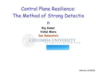
Theoretical Bounds on Control Plane Monitoring in Routing Protocols Dan Rubenstein. Joint work with Raj Kumar, Vishal Misra. Routing Protocols with Misconfigurations. Routing Protocols in “friendly” environments are well understood, e.g., Link State: global knowledge, centralized approach

E N D
Theoretical Bounds on Control Plane Monitoring in Routing Protocols Dan Rubenstein Joint work with Raj Kumar, Vishal Misra
Routing Protocols with Misconfigurations • Routing Protocols in “friendly” environments are well understood, e.g., • Link State: global knowledge, centralized approach • Distance Vector (a.k.a. Bellman-Ford): known to converge (quickly), adapt to changes, etc. • BGP (Path-Vector): some problems in converging when routes change, significant literature evaluating/understanding • Critical Assumption for correctness: Nodes follow the proper protocol procedure • Q: What happens when nodes don’t follow the protocol like they’re supposed to?
8765 7007 7074 6957 5165 2134 4345 History Shows: Misbehaving nodes can be a big problem • The infamous BGP AS 7007 Incident (& Pakistan YouTube): • Consider routes to node 8765 (all edges length 1) … Traffic goes where it is supposed to
8765 7007 7074 6957 5165 2134 4345 Nodes don’t always “behave” • The infamous BGP AS 7007 Incident: … Traffic enters “black hole”
The Future of Distributed Routing Protocols • Controlled environments (e.g., Intra-domain Internet) have moved away from distributed routing protocols toward “link-state” • But other future networks are expected to rely on distributed routing solutions: • Ad hoc networks • Sensor networks • DTNs • Mesh networks • Our formal approach: start by understanding the self-monitoring capabilities of well-known distributed routing protocols
Can I tell if my neighbors are giving me the correct information? A Theory to detect “Bad” Nodes • Rules: • “Bad” nodes misinform, “Good” nodes can attempt to detect the bad nodes • “Good” nodes are limited to information provided by the routing protocol • Want to exchange additional info, modify the protocol • Challenge: When can a good node determine something isn’t right?
A B D E A Node’s Info: Its State • A node’s state is its (only) view of the network • e.g., Distance-Vector (a.k.a. Bellman-Ford) C F G Note our convention: (I,J) in state table reports node I’s distance to J (not local node’s distance to J through I)
N X Y N X Y 1 3 Detection • Assume: Routes have stabilized (routing protocol inactive) • Q: For routing protocol P, given a good node’s state, what misconfigurations can it detect/observe within the network? • Note: A node can’t always detect a problem D(X,Y) = 3 1 1 An undetectable misconfig at node N:
Prior Work • Some work verifying the data plane: • [MCMS’05]: addresses subversion of forwarding process (routers don’t forward packets as specified in control plane) • Some work modifying protocols to explicitly facilitate detection of misbehaving nodes; • [SRKSS’04]: Listen & Whisper • [HPS’05]: Secure BGP • [LSP’82]: Byzantine Generals’ Problem: determine who in a group is lying
Prior Work: “Weak” Detection • Process for constructing a weak detection method: • Find a property that a node’s state should exhibit • Check the property in a node’s state • Declare misconfiguration in network if property is violated • A detection method is “Weak” if it fails to identify a misconfiguration that is detectable using another method (on same state)
A Weak Detection Method: Symmetry • In an undirected graph, D(X,Y) = D(Y,X) • Here, D(A,B) = 1 • But D(B,A) = 4 • Using Symmetry, found a misconfiguration • So why is Symmetry weak?
Another Weak Detection Method: Triangle Inequality [DMZ’03] • Triangle inequality should hold: D(X,Z) ≤ D(X,Y) + D(Y,Z) • Violated here: • D(B,E) = 3 • D(B,A) = 1 • D(A,E) = 1 • D(B,E) > D(B,A) + D(A,E) • Note: symmetry property not violated • Example shows why detection via symmetry is weak: failed to identify a detectable misconfiguration • So why is triangle inequality weak?
D Weakness of Triangle Inequality A • Suppose graph edge lengths are all 1 • No violation of symmetry or triangle inequality C B Where to place edges? A and B are our neighbors C is distance 1 from B D is distance 3 from both A & B: nowhere to put connecting edge
“Strong” Detection • A detection method is “strong” if it always detects detectable misconfigurations • More formally, Let • μ be a method to detect misconfigurations • C = {N} be the set of valid networks (what the network might look like) • NRbe the actual network (Note NRє C) • sn(N) be the state of node n when the routing protocol is executed correctly (and stabilized) within a network N є C • s’n(NR) be the state actually computed at node n (possibly with misconfigurations) in network NR • Node n knows s’n(NR), C, and given N є C, can compute sn(N) • Node n does not know NR or sn(NR) • μ is a strong detection method if one of the following holds whenever s’n(NR) ≠ sn(NR) (n’s state affected by misconfiguration): • Detected: μ detects that sn(NR) ≠ s’n(NR) • Undetectable: No method μ’ exists that can detect sn(NR)≠s’n(NR)
A High-Complexity Strong Detection Algorithm • Input: • State s’n(NR) of node n for the “real” but unknown network NR • Description of set of allowable networks, C = {N} • Algorithm: For each N є C • Compute sn(N) (n simulates protocol on N) • If sn(N) = s’n(NR) then return MISCONFIG UNDETECTABLE (N might be the valid network) • If no N є C matches, then MISCONFIG DETECTED Algorithm Complexity is ~C, often huge or infinite!
Low-Complexity Strong-Detection • Q: Can Strong Detection be achieved with low complexity? • A: Sometimes: we show how to do it for Bellman-Ford (a.k.a. Distance Vector) and variants of Path Vector (simplified BGP)
Strong Detection for D.V. • Input at node n: • S’n(NR): a single node’s (steady state) state table that reports each neighbor’s (supposed) distance to all nodes • Set C of all allowable networks • defined by {Axy}: Axy is the set of allowable lengths of edges between node x and y • Axy can be any union of intervals that are closed from below • e.g., Axy = [0,3) U [4,4] U [7,100] • Other more common examples: • Axy = [0,] • Axy = [1] U [] S’n(NR)
D F G A B C n G E B C n E F D A G Strong Detection in D.V. at a node, n • Take node n’s state, s’n(NR) • Use this state to build the canonical graph, G є C • Simulate D.V. on G to generate simulated state sn(G) • We will prove: • If sn(G) ≠ s’n(NR), then misconfiguration detected • Else, either there is no misconfiguration, or it is undetectable (using node n’s state) because G might be the actual network s’n (NR) sn(G)
Creating the Canonical Graph, G for an undirected network • For each pair of nodes (x,y): • Create edge (x,y) with length exy = smallest value in Axy ≥ maxm є V(n) |d(m,x) – d(m,y)| • exy = ∞ if all values in Axy too small • Consider state table on left • eCD ≥ max(|12-5|, |13-9|, |8-12|) = 7 • If ACD = [1,1] U [4,6] U [8,10], then eCD = 8
Proving Strongness of the Canonical Graph Method • N: a network for which sn(N) = s’n(NR), when such a network N exists • G: the canonical graph constructed by n from s’n(NR) • fxy: length of edge (x,y) in N (when the edge exists) • exy: length of edge (x,y) in G (edges always exist) • dH(x,y): shortest path distance from x to y in a network H • Assume: all edges have positive length (easy to extend when edges can also have length 0) • High Level Sketch of Proof: • If N exists where sn(N) = s’n(NR), then sn(G) = sn(N) = s’n(NR) • If N does not exist, then sn(G) ≠ s’n(NR)
n v y x fxy Bounds on exy • Lemma 1: If sn(N) = s’n(NR) for some N є C and edge (x,y) exists in N with length fxy, then exy ≤ fxy(Canonical Graph Edges Never Longer) • Proof: In N, x & y’s distances to any neighbor v must differ by at most fxy, i.e.: For each neighbor v, |dN(v,y) – dN(v,x)| ≤ fxy • Hence maxm є V(n) |d(m,x) – d(m,y)| ≤ fxy • Recall exy = smallest value in Axy ≥ maxm є V(n) |d(m,x) – d(m,y)| • Since N є C, we have fxy є Axy and so exy ≤ fxy
x n Shortest Path P from v to x in N • Lemma 2: If sn(N) = s’n(NR) for some N є C, then dN(v,x) ≥ dG(v,x) for all neighbors v and all nodes x (Canonical Graph Shortest Paths are never longer) • Proof: • Choose any neighbor v to any node x, and choose any shortest path P from v to x in N • By Lemma 1, each edge (a,b) N satisfies eab≤ fab • The path P through the same set of nodes can’t be longer in G than in N • So there is a shortest path in G from v to x no longer than the path in N v x Path P from v to x in G
in N: v y y exy x n exy < | dN(v,x) - dN(v,y) | exy ≥ |dN(v,x) – dN(v,y)| Blue nodes t satisfydG(v,t) < dN(v,t) • Lemma 3: If sn(N) = s’n(NR) for some N є C, then dG(v,x) ≥ dN(v,x) for all neighbors v and all nodes x (Canonical Graph Paths never shorter) • Proof: by contradiction. Select x with smallest dG(v,x) where dG(v,x) < dN(v,x) • Let y be the node preceding x on a shortest path from v to x in G where edge exy connects y to x on this path • hence dG(v,y) < dG(v,x) and exy = dG(v,x) - dG(v,y) (equality because exy is on x’s shortest path through y) • dG(v,y) < dG(v,x), hence y not blue dG(v,y) ≥ dN(v,y) • Hence exy = dG(v,x) - dG(v,y) < dN(v,x) - dN(v,y) = | dN(v,x) - dN(v,y) | x Distance from v in G But exy constructed = maxm |dN(m,x) – dN(m,y)|, and maxm |dN(m,x) – dN(m,y)|≥ |dN(v,x) – dN(v,y)| !!
The Main Result • Some N є C produces state sn(N) = s’n(NR) sn(G) = s’n(NR) • Proof: • Follows from Lemma 2 (dG(v,x) ≤ dN(v,x))and Lemma 3(dG(v,x) ≥ dN(v,x)) • If no N є C produces state s’n(N), since G є C, G cannot produce state = s’n(N) • In other words, only need to check if sn(G) = s’n(NR) • Complexity: O(|V|3) • Construct the canonical graph, G • Simulate Bellman-Ford • Compare State Tables
D(a,b)=y x b a monitor liar Lied-about Simulation Results Simulation 1 • How big does an error have to be before it is detected? • Define Detection Threshold: max % change liar can make in distance report w/o getting caught. • As function of monitor-liar distance for single and multiple errors • Used topologies generated via BRITE Detection is clearly function of distance
D(a,b)=y x b a monitor liar Lied-about Simulation Results cont’d Simulation 2 • How do distances affect detection? • Monitor-Liar • Liar–Lied About • Monitor–Lied About Monitor-Liar distance most correlated with detection
Path Vector Protocols (e.g., BGP) • Node state contains information about entire path to destination. We consider 2 variants: • V1: Each hop + link weight per hop given • V2: Each hop + total path length given • Strong Detection Result: • V1: trivial to either find conflict, else state itself is feasible construction • V2: State can be viewed as linear program: • Path Pi formed by edges (xi1, xi2, …, xik) has length yi • Equation in linear program: xi1 + xi2 + … xik = yi • Strong Detection approach: determine existence of solution to linear program • Solution exists cannot detect • No solution exists misconfiguration
Extensions / Future Directions • Same idea works for: • Directed graphs • Using state info from a set of trusted nodes • Future Directions: • Identifying the offending node (not just its existence) • Performing Strong Detection for other routing protocols (Ad-hoc network, geographical positioning) • See our paper in Sigmetrics’07