Download
1 / 10
100 likes | 190 Views
Chapters 16, 17, and 18. Expected value Law of Averages Central Limit Theorem. Box Models. Flipping a coin n times, or rolling the same die n times, or spinning a roulette wheel n times, or drawing a card from a standard deck n times with replacement , …

E N D
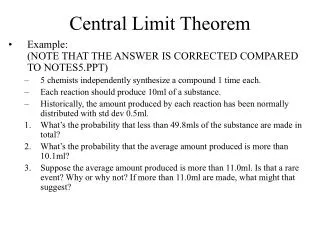
Chapters 16, 17, and 18 Expected valueLaw of Averages Central Limit Theorem
BoxModels • Flipping a coin n times, orrolling the same die n times, or spinning a roulette wheel n times, or drawing a card from a standard deck n times with replacement, … • Interested in the accumulation of a certain quantity? We can box model the process. • Actual outcomes are therefore abstractly represented by tickets.
How to Make a Box Model • First draw a rectangular box. • Then write next to the box how many times you are drawing from it: n = … • What tickets go inside the box? • That depends on what valueyou could add on to a requested quantity each time you draw from the box! • Then, write the probability of drawing a particular ticket next to that ticket. • Examples: Chapter 16, #5-8
ExpectedValue • The expected value of n draws from the box is therefore given by: • EVn = n*EV1 • The expected value of 1 draw from the box, also called the box average, is given by: • EV1= weighted average of tickets in box • = first ticket *probability of drawing first ticket + second ticket *probability of drawing second ticket + …
Law of Averages • “The more you play a box-model-appropriate game, the more likely you get what you see of the box.” • “What is expected to happen will happen.” • Examples: Chapter 16, #1, #4 • A consequence of the Law of Averages is that we should not hope to come away with a gain by playing many times – we will eventually come out as a loser if we play long enough.
Standard error • The expected value of n draws is given by EVn = n*EV1, where EV1 is the average of the box. • Now of course our actual accumulated total could differ somewhat from the expectation, and we call our typical deviation standard error, given by: • SEn = √n *SE1, where SE1 is the standard error of the box.
Standard error of a box • Standard error of a box, or standard error of a single play, or standard error of a single draw, all mean the same thing. • For a box with only two kinds of tickets, valued at A and B respectively, and with probability of p and q of being drawn respectively, the standard error of the box is given by: • SE1=|A-B|* √(p*q) • Examples: Chapter 17 #10
ContinuityCorrection • This is related to the normal table we played with. • Now the EVn acts as the “Average” • And SEn acts as the “Standard Deviation” • Chapter 17, Question 3c • Continuity Correction is needed when you are dealing with discrete outcomes. • Suggestion: Draw the normal curve and label the average. Then judge where you want to be and in what direction you should shade; then standardize and look up percentages. • And so the new version of Standardization Formula:
C.C. and Discrete Outcomes • When do we know we may use continuity correction? • That’s when the observed outcomes are discrete. • For example, if you are counting the number of democrats among a sample of 400 people, you can probably get 0, 1, 2, …, 399 ,or 400, but nothing else between any two numbers (such as 349.97) • Examples: All questions in Chapter 18 where the box model is a “COUNTING BOX” (box with only 0 and 1) • A non-example: Height of people in the US • Example: P(at least break even) = P(actual > -0.5) • Example: P(lose more than $10) = P(actual < -10.5) • Example: P(win more than $20) = P(actual >20.5) • Example: P(no more than 2300 heads) = P(actual < 2300.5)
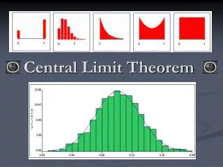
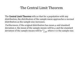
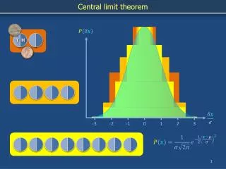
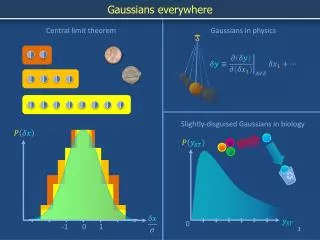
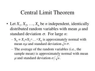
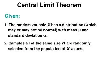
Central limit theorem (CLT) • The basis for what we did is called Central Limit Theorem. • The Central Limit Theorem (CLT) states that if… • We play a game repeatedly • The individual plays are independent • The probability of winning is the same for each play • Then if we play enough, the distribution for the total number of times we win is approximately normal • Curve is centered on EVn • Spread measure is SEn • Also holds if we are counting money won • Note: CLT only applies to sums! See Chapter 18 Question 10.