Download
1 / 40
400 likes | 631 Views
Using Pulsars to probe the interstellar medium. Barney Rickett, University of California San Diego Department of Electrical & Computer Engineering. Presentation at PAC 2012 - KIAA/PKU October 2012. Probing the Galaxy with Pulsars big picture.

E N D
Using Pulsars to probe the interstellar medium Barney Rickett, University of California San Diego Department of Electrical & Computer Engineering Presentation at PAC 2012 - KIAA/PKU October 2012
Probing the Galaxy with Pulsarsbig picture • FAST sensitivity and sky coverage => More pulsars and DMs (DM = ∫ ne dl) • Pulsar HI absorption measurements => new pulsar distances • More pulsars, DMs & distances • => Better model for electron distribution in Galaxy • => Better model for 3D distribution of pulsars • Pulsar Rotation Measures + better electron model • => Better model for Galactic Magnetic Fields
DM sin(b) versus Latitude bassume stratified disk => electron density ne(z) • DM = ∫ Lp ne dl = ∫ Zp ne(z) dz/sinb • DM sinb = ∫ Zpne(z)dz • if Zp < Hne DM => Lp ne(0) Lp • if Zp > Hne DM sinb => DM90 = ∫ ∞ne(z)dz ~ ne(0) Hne z * Zp Hne Lp * ne(z)
20/sinb DM versus Latitude b DM = ∫ ne dl = ∫ ne(z)dz/sinb < DM90 /sinb
DM sin(b) versus Latitude DM sinb = ∫ Zpne(z)dz < DM90
Delay spectrum (Jenet et al. 2010) PSR B1937+21 Possibility to determine the temperature and number of cool HI clouds. emission absorption delay
H-a Galactic Distribution Cygnus Region SMC LMC Ia ~ ∫ ne2 dl = EM (cm-6 pc) Large Iacan be a lower bound to EM (due to saturation)
FAST: ZA< 40deg AO: ZA< 20deg Psrs & high DM in LMC & SMC Pulsar DMs + Galaxy Ha
FAST: ZA< 40deg AO: ZA< 20deg Zoom Pulsar DMs + Galaxy Ha
Probing the Galaxy with Pulsars • Modelling the electrons in the Galaxy: • Taylor & Cordes 1993; Cordes & Lazio 2001-2006 • Questions: • Are pulsars concentrated in spiral arms? • At 100 km/sec a psr moves 1kpc in 107 years • Is the concentration of psrs near 40deg longitude: • a spiral arm? or due to AO observational (sensitivity) bias • What is ne between the spiral arms? • Are there more pulsars hidden by scattering in the Cygnus region? • Better estimates of the perpendicular distribution of pulsars & electron density
Spiral structure 42 deg Cordes & Lazio 2006
Cordes Lazio Ne model (~2006) Need to compare distributions of Plasma and Pulsars Neutron star distribution as history of star formation ?
Probing the Galaxy with Pulsarssmall-scale picture • Small-scale structure in the ISM scatters radiowaves • Refractive index deviation l2 • Scattering is typically consistent with Kolmogorov turbulence over scales from 1000 km -> 100 AU (Armstrong et al. 1995) • But turbulence level is very inhomogeneous i.e. “patchy” • see the Ha maps • Turbulence is often anisotropic • Probe by pulsar scattering: • DM variation • Pulse Broadening time & ISS bandwidth • Scattering hides pulsars (esp. MSPs) • Scintillation Arcs (Stinebring et al.)
ISS Geometry From Radio Galaxy Quasar or AGN 2000 pc
The solid line gives the best fit line with power law index a =1.66 ±0.04 consistent with Kolmogorov a = 5/3 Ramachandran et al 2006: Slope = 1.66 Structure function of Dispersion Measure PSR B1937+21Ramachandran et al. 2006
pulsar Temporal broadening zp scattering layer zo q Scattered Image Brightness = B(q,b) Scattered Pulse shape: P(t) = ∫ 02πB[q=√(2ct/zeff),b] db zeff = (zo+zp)(zp/zo) Pulse Broadening timetscatt= zeffq2 /2c f -4.4
Scattered pulse shape for PSR J1644-45 observed at 660 MHz at ParkesRickett, Johnston and Tomlinson, 2004 Kolmogorov: Inner scale < 10km loge[P(t)] Detailed shape is a diagnostic of scattering at high wavenumbers (ie due to very small scales) Conclude linner ~ 75 km Allowing for anisotropy makes this a lower limit This requires very high signal to noise ratio (ie FAST) Inner scale > 1000km
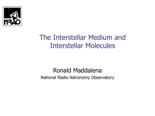
The uniform Kolmogorov model predicts:tscatt DM2.2 But the observations show a much steeper dependence on DM. They imply that at larger distances through the electron layer, there is an increasing chance of encountering regions of high density and high turbulence. This result is built in to the Galactic electron model of Cordes & Lazio (2003) as a high level of patchy turbulence in the inner Galaxy tscatt versus DM Note that tscatt responds to a column of density-variance (related to emission measure). Since we expect dne ~ne , tscatt picks out the highest densities along a line of sight.
dnd PSR B1133+16 at Arecibo(Stinebring et al.) Scintillation Arcs dtd tscatt= 1/(2π dnd) “Secondary Spectrum” (S2) with three scintillation arcs Primary Dynamic Spectrum
delay t (µsec) Doppler Frequency fD (mHz) The Puzzle of the “Arc-lets” Hill, Stinebring et al. (2005) showed this example of the arcs observed for pulsar B0834+06. In addition to the main forward arc (following the dotted curve) there are “reverse arclets”. Those labelled a-d are particularly striking. They observed them over 25 days and found that they moved in Delay and Doppler, precisely as expected for the known pulsar proper motion.
The Puzzle of the “Arc-lets” 2 Doppler Frequency fD (mHz) 334 MHz 321 MHz Predicted for plasma refraction The right plot shows how fD varies with observing frequency. Remarkably this shows that the spatial location of the scatterers is independent of frequency. They DO NOT show the expected shift due to the dispersive nature of plasma refraction. The left plot shows the angular position of the structures (in mas) responsible for each reverse arclet, mapped from the Doppler frequency fD . The lines have the slope expected for the known pulsar proper motion.
Note reverse arclets and one group at delay of 1 msec VLBI of Scintillation Arcs (Brisken et al 2010)
Note the faint offset scattering responsible for the “1 msec” arclet Scattered Brightness from B0834+06 Scattered image reconstructed by mapping from the secondary spectrum. The phase provides orientation in RA/Dec (J-J Gao PhD UCSD) Dqdec (mas) DqRA (mas)
Walker’s decomposition of Hill/Stinebring observations of B0834+06 327 MHz Arecibo Imaged by Gao assuming Vpsr Doppler Frequency fD (mHz) Blue line shows the axis derived from VLBI by Brisken, Gao et al. Scattered Brightness is Anisotropic, Asymmetrical & Intermittent
New tool for study of ISM • Thin screen model is often remarkably successful => ISM is patchy • Examples of thin arcs and multiple “reverse arclets” require: • a) Highly anisotropic scattering • b) very patchy distribution of “turbulence” • Intense turbulent regions ~10 AU dominate in a path of 108 AU ! • Together these upset the assumptions of isotropy and uniformity in a turbulent & ionized ISM. Instead we have anisotropy and intermittency in the turbulence. • It leaves us with fascinating puzzles: • What are the astro-physical sites that cause peaks in the scattering? • What is the cause of the 1-D fine structure ? What role for magnetic field? • What consequences for MSP timing ? • New ideas from Cyclo-Stationary spectral analysis • New facilities GBT, EVLA, LOFAR, FAST What do arcs tell us?
The sensitivity of the FAST telescope will explore the ISM on the large scale: • Spatial distribution of Pulsars • Inside and outside of spiral arms • More associations with supernova remnants • New distance measurements by sensitive HI absorption • Delay spectrum as a new probe of HI • New DMs improve the modelling of plasma in the Galaxy (Ne2020?) • What ionizes the ISM? • Influence of HII regions and supernova remnants • New Rotation Measures improve knowledge of the Galactic Magnetic Field • RM from pulsars, extra-galactic sources and diffuse synchrotron emission Scattered pulse shapes and secondary spectra will explore the ISM on the small scale: • Monitoring the non-uniform ISM for corrections to pulsar timing • DM variation of MSPs for timing correction • Particular discrete regions of scattering • What is their physical origin? • What is their density in interstellar space? • Study of turbulence in the interstellar plasma Summary
PSR B1737+13 mjd 53857 Arecibo 320 MHz Stinebring In the 1-D scattering we find secondary spectrum: S2(t,fD) µ B(t/AfD+AfD) x B(t/AfD-AfD) / |fD| in terms of the 1-D brightness function B(q) and a scaling constant A Hence from observations of S2 one can fit the observations S2 to a 1-D model and so estimate B(q)
PSR B1737+13 mjd 53857 1700 MHz 1-dim Scattered Power Scattered Brightness is Anisotropic, Asymmetrical & Intermittent
ft Relative to a center time t0 and frequency n0, the interference term is: Cos[2πfn(n-n0) + 2πft(t-t0)+Df0] fn = dt1- dt2 = [q12- q12] (z/2c) ft = dn1- dn2 = (q1x- q2x)V/l t-t0 fn 2DFT x x S1 S2 n-n0 scattering screen Secondary spectrum theory 1 I = |E1 + E2|2 if E1 and E2 are coherent at frequency n: = |E1|2 + |E2|2 + 2E1E2cos(Df) where Df = 2π(n1t1-n2t2)+f01-f02 t1 = t+dt1 ,n1 = n+dn1 Df = 2π[n(dt1- dt2)+(dn1- dn2)t .. + ..O(dn,dt) + f01-f02] V where dt1 = zq12/2c is the relative time delay dn1 = n(V.q1)/c is the relative Doppler frequency
V q 2 z q 1 scattering screen Arc Equations t= dt1- dt2 = [q12- q22] (z/2c) fD = dn1- dn2 = (q1x- q2x)V/l With q2 fixed there is a quadratic relation between t and fD which depends on q1y2. If in addition q1x and q1y lie on a straightline (ie 1-D scattered brightness) the relation is a parabola through the origin => reverse arclet b In that case the visibility phase on baseline b corresponds to the mean position of the two angles => π (q1+ q2). b/l Apex of parabola is where q2=0, hence visibility phase at an apex gives astrometric measure of q1.
B1737+13 10-weeks of 1-D models Proper motion ~30 mas/yr Psr distance 4.8 kpc (DM) Angle units ~ mas Proper motion predicts 0.5 mas per week No coherent shifts seen Some decorrelation even over half-hour
Alternative Geometries for Arcs Individual scattering centers Background of distributed turbulence Perpendicular Geometry Anisotropic & intermittent - spaghetti-like filaments in SN remnants Separate offset feature also needed Parallel Geometry Isotropic scatterers clumped linearly Other clumps too far from line of sight
Part of Cygnus Loop Supernova Remnant age 5-10 Kyr ~4 pc Bright shell: EM ~ 100 pc cm-3 dL ~ 1 pc => max ne ~ 10 cm-3
Density of Galactic plane pulsars vs longitude Ha intensity ± 5 deg latitude