Download
1 / 47
540 likes | 834 Views
Chapter 7. Database Languages. The Relational Algebra. The relational Algebra. The relational algebra is a complete set of operations on relations which allows to select data from a relational database. Cartesian product Union , Intersection , Difference Projection q -join Division.

E N D
Chapter 7 Database Languages
The relational Algebra • The relational algebra is a complete set of operations on relations which allows to select data from a relational database. • Cartesian product • Union , Intersection , Difference • Projection • q-join • Division
Sample database R r1 r2 r3 S1 s1 s2 1 x 3 3 p 4 x 3 4 q 3 y 4 4 p 2 z 7 S2 s1 s2 4 q 2 m
Cartesian product R x S2 r1 r2 r3 s1 s2 1 x 3 4 q 4 x 3 4 q 3 y 4 4 q 2 z 7 4 q 1 x 3 2 m 4 x 3 2 m 3 y 4 2 m 2 z 7 2 m
Projection , q -join Projection R [ r2 , r3 ] r2 r3 x 3 y 4 z 7 q-join R [ r3 > s1 ] S1 r1 r2 r3 s1 s2 3 y 4 3 p 2 z 7 3 p 2 z 7 4 q 2 z 7 4 p
Left Outer-join R[r3 =ls1]S1 r1 r2 r3 s1 s2 1 x 3 3 p 4 x 3 3 p 3 y 4 4 q 3 y 4 4 p 2 z 7
Union , Intersection , Difference s1 s2 3 p 4 q 4 p 2 m UNION S1 ÈS2 s1 s2 4 q Intersection S1 ÇS2 s1 s2 3 p 4 p Difference S1 \ S2
Division Divide by ÷ Result DEND/DOR DEND P# p1 S# s1 s2 DOR 1 S# P# s1 p1 s1 p2 s1 p3 s1 p4 s1 p5 s1 p6 s2 p1 s2 p2 s3 p2 s4 p2 s4 p4 s4 p5 P# p2 p4 S# s1 s4 DOR 2 P# p1 p2 p3 p4 p5 p6 DOR 3 S# s1
S S# Sname 1 Jones 2 Duval 3 Codd 4 Carter SP S# P# 1 11 1 15 2 12 3 15 1. Give all parts 2. Give names of suppliers supplying part 15 3. Give those suppliers that do not supply part 15 4. Give those suppliers that supply something else than part 15 5. Give those suppliers that supply something but not part 15 Example
Solutions 1. SP [ P# ] 2. ( ( S [ S# = S# ]SP )[ P# ÷ 15] [15 ]) [ Sname ] 3.
Sample Database S S# SNAME STATUS CITY S1 Smith 20 London S2 Jones 10 Paris S3 Blake 30 Paris S4 Clark 20 London S5 Adams 30 Athens • SP S# P# QTY • S1 P1 300 • S1 P2 200 • S1 P3 400 • S1 P5 200 • S1 P6 100 • S2 P1 300 • S2 P2 400 • S3 P2 200 • S4 P2 200 • S4 P4 300 • S4 P5 400 • P P# PNAME COLOR WEIGHT CITY • P1 Nut Red 12 London • P2 Bolt Green 17 Paris • P3 Screw Blue 17 Rome • P4 Srew Red 14 London • P5 Cam Blue 19 London • P6 Cog Red 19 London
Create Table CREATE CREATE TABLE base-table-name ( base-table-element - commmalist ) where base-table-element is a column-definition or a base-table-constraint-definition column-definition: column representation [ default definition ] default definition: NOT NULL, NULL, current-date, ....)
Base-table-constraint • candidate key: UNIQUE ( column-commalist ) • primary key: PRIMARY KEY ( column-commalist ) • foreign key: FOREIGN KEY ( column-commalist ) REFERENCE base-table [ ( column-commalist ) ] [ ON DELETE option ] [ ON UPDATE option ] option: NO ACTION , CASCADE, SET DEFAULT, SET NULL • check constraint: CHECK ( conditional-expression )
CREATE table example CREATE TABLE SP (S# S# NOT NULL, P# P# NOT NULL, QTY QTY NOT NULL, PRIMARY KEY ( S# , P# ) FOREIGN KEY ( S# ) REFERENCE S ON DELETE CASCADE ON UPDATE CASCADE, FOREIGN KEY ( P# ) REFERENCE P ON DELETE CASCADE ON UPDATE CASCADE, CHECK ( QTY > 0 AND QTY < 5001 ) ) ;
DDL - table modification ALTER table ALTER TABLE base-name-table ADD column-name data-type ; ( “not null” is not permitted ) DROP table DROP TABLE base-table-name
DDL - Indexes CREATE index CREATE [ UNIQUE ] INDEX index-name ON base-table-name ( column-name [ ORDER ] [ , column-name [ ORDER ] ... ) DROP index DROP INDEX index-name ;
DML - Data Manipulation Language SQL SELECT [ DISTINCT ] field(s) FROM table(s) [ WHERE predicate ] [ GROUP BY field(s) [ HAVING predicate ] ] [ ORDER BY field(s) ] ;
Simple Retrieval - SQL Get part numbers for all parts supplied SELECT P# FROM SP ; SELECT DISTINCT P# FROM SP ; P# P1 P2 P3 P4 P5 P6 P1 P2 P2 P2 P4 P5 P# P1 P2 P3 P4 P5 P6
Simple retrieval - QBE Get part numbers for all parts supplied SP S# P# QTY P._PX SP S# P# QTY P.ALL._PX
Retrieval of expressions For all parts get the part number and the weight in grams ( in the table weights are in pounds ). SELECT P.p# , P.weight*454 FROM P ; OUTPUT P# P1 5448 P2 7718 P3 7718 P4 6356 P5 5448 P6 8626 P P# Pname Color weight City P._PX P.Weight *454
Simple retrieval of table Get full details of all suppliers SELECT * FROM S ; SQL QBE S S# Sname Status City P._SX P._SN P._ST P._SC S S# Sname Status City P.
Qualified retrieval 1 Get supplier numbers for suppliers located in Paris or with status greater than 20. SELECT S# FROM S WHERE City = ‘PARIS’ OR Status > 20 ; S S# Sname Status City P._SX > 20 P._SY Paris
Qualified retrieval - 2 Get supplier numbers for suppliers located in Paris with status greater than 20. SELECT S# FROM S WHERE City = ‘PARIS’ AND Status > 20 ; S S# Sname Status City P._SX > 20 Paris
Qualified retrieval with ordering Get supplier numbers and status for suppliers in Paris in descending order of status SELECT S# , Status FROM S WHERE City = ‘Paris’ ORDER BY Status DESC ; S S# Sname Status City P._SX P.DO._ST Paris
Simple Equi-join Get all combinations of supplier and part information such that the supplier and part in question are located in the same city SELECT S.* , P.* FROM S , P WHERE S.City = P.City ; SQL QBE S S# Sname Status City P. _X P P# Pname Color weight City P. _X
Greater-than join Get all combinations of supplier and part information such that the supplier city follows the part city in alphabetical order. SQL SELECT S.* , P.* FROM S , P WHERE S.City > P.City QBE S S# Sname Status City P. > _X P P# Pname Color weight City P. _X
Join with additional condition Get all combinations of supplier and part information such that the supplier and part are colocated , but omitting suppliers with status > 20 . SQL SELECT S.* , P.* FROM S , P WHERE S.City = P.City AND S.Status NOT > 20 ; QBE S S# Sname Status City P. NOT > 20 _X P P# Pname Color weight City P. _X
Retrieving specified fields from a join Get all part-number / supplier-number combinations such that supplier and part are colocated SQL SELECT S.S# , P.P# FROM S , P WHERE S.City = P.City QBE S S# Sname Status City P._SX _X P P# Pname Color weight City P._PX _X
Join of three tables Get all pairs of city names such that a supplier located in the first city supplies a part stored in the second city SQL SELECT DISTINCT S.City , P.City FROM S , P , SP WHERE S.S# = SP.S# AND SP.P# = P.P# ; QBE S S# Sname Status City SP S# P# QTY _X _Y _X P._CS P P# Pname Color weight City _Y P._PC
Function in a select clause Get the total number of suppliers SQL SELECT count ( * ) FROM S ; QBE S S# Sname Status City P.COUNT._SX
Function in select clause with predicate Get the total number of suppliers supplying part 2. SQL SELECT count ( * ) FROM SP WHERE P# = ‘P2’ ; QBE SP S# P# QTY P.CNT.ALL._SX P2
Join of table with itself Get all pairs of supplier numbers such that the two suppliers are colocated . SELECT FIRST.S# , SECOND.S# FROM S FIRST , S SECOND WHERE FIRST.City = SECOND.City AND FIRST.S# < SECOND.S# ; S S# Sname Status City _SX _SY _CZ _CZ Conditions _SX < _SY RESULT FIRST SECOND P. _SX _SY
Use of GROUP BY For each part supplied , get the part number and the total shipment quantity for that part SQL SELECT P# , SUM(QTY) FROM SP GROUP BY P# ; QBE SP S# P# QTY P.G._PX P.SUM.ALL._QX
Use of HAVING Get part numbers for all parts supplied by more than one supplier. SQL SELECT P# FROM SP GROUP BY P# HAVING COUNT(*) > 1 ; QBE SP S# P# QTY _SX P._PX NOT._SX _PX or SP S# P# QTY CNT.ALL._SX> 1 P.G._PX
Retrieval involving a subquery Get supplier names for suppliers who supply part P2 . SELECT Sname FROM S WHERE ‘P2’ IN (SELECT P# FROM SP WHERE S#= S.S#) ; SELECT UNIQUE SNAME FROM S , SP WHERE S.S# = SP.S# AND SP.P# = ‘P2’ ; SELECT UNIQUE Sname FROM S WHERE S# IN (SELECT S# FROM SP WHERE P# = ‘P2’) ; S S# Sname Status City _X P._SN SP S# P# QTY _X P2
Single-record Update Change color of part P2 to yellow SQL: Update distinct P Set color = “yellow” where P# = P2 ; QBE: P p# pname color weight city p2 U.yellow
Multiple Update Double the status of all suppliers in London SQL Update S Set status = status * 2 where City = “London” ; QBE S S# sname status city _SX _ST London U. _SX 2 * _ST
Update involving sub-query Set quantity to zero for all suppliers in London Update SP Set qty = 0 where “London” = ( select city from S where s# = SP.s# ) ; SQL QBE SP s# p# qty U. _SX 0 S s# sname status city _SX London
Views CREATE VIEW name AS SELECT statement ; Example: CREATE VIEW good-suppliers AS SELECT s# , status , city FROM S WHERE status = 15 ; The VIEW-definition is stored in the directory but the select is not performed
VIEWS - 2 Example: CREATE VIEW PQ ( P# , sumqty ) AS SELECT p# , SUM(qty) FROM SP GROUP BY p# ; • Views can be defined in terms of other views • Some views are updateble • Views can be dropped
VIEWS - usage VIEWS can be used just like base tables CREATE VIEW LONDON-SUPPLIERS AS SELECT s, sname , status FROM S WHERE city = ‘London’ ; Two formulations with the same result SELECT * SELECT s# , sname , status FROM LONDON-SUPPLIERS FROM S WHERE status < 50 WHERE status < 50 ORDER by s# ; AND city = ‘London’ ORDER BY s# ;
SQL System Catalog The system catalog is also a relational database SYSTABLES ( name , creator , colcount , ... ) SYSCOLUMNS ( name , tbname , coltype , ... ) SYSINDEX ( name , tbname , creator , ... ) Examples: SELECT tbname FROM SYSCOLUMNS WHERE name = ‘s#’ ; SELECT name FROM SYSCOLUMNS WHERE tbname = ‘S’ ; Updating the catalog is not possible
QBE dictionary Retrieval of table names : Get all tables known to the system P. Creation of new table I. S S# Sname Status City I. S S# Sname Status City domain S# Sname Status City type char 5 char 20 fixed char 15 key Y U.N U.N U.N invers Y U.N U.N U.N