Download
1 / 21
210 likes | 333 Views
Elasticity, price changes, and changes in total revenue (TR) (total expenditure, (TE)). In the market for a particular good: Total revenue (TR) is the amount of money sellers take in. Total expenditure (TE) is the amount of money buyers pay out. Assuming no excise taxes:

E N D
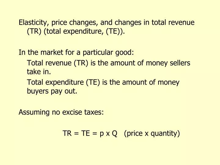
Elasticity, price changes, and changes in total revenue (TR) (total expenditure, (TE)). In the market for a particular good: Total revenue (TR) is the amount of money sellers take in. Total expenditure (TE) is the amount of money buyers pay out. Assuming no excise taxes: TR = TE = p x Q (price x quantity)
p p2 TR2 = p2 x Q2 TR1 = p1 x Q1 p1 Demand Q1 Q Q2 Question: When p and Q change as the result of movements along a demand curve, what is the relationship between changes in price and changes in TR? When p increases, Q decreases, so it’s not clear, without more information, how TR is affected. Need info about elasticity of demand.
“big” increase in p . . . combined with “small” decrease in Q TR = TE increases, on balance. Let’s look at some cases: Suppose demand is inelastic (%Q < %p) and price increases (quantity decreases). (Keep in mind -- we’re talking about movements along a demand curve.) TR = TE = p x Q
p p2 p1 Q1 Q2 Q This is easy to remember by visualizing a demand curve close to the limiting case of perfectly inelastic: For a demand curve that is close to perfectly inelastic, it’s obvious that TR = TE increases when price increases.
“small” increase in p . . . combined with “big” decrease in Q TR = TE decreases, on balance. Now suppose that demand is elastic (%Q > %p) and price increases (quantity decreases). TR = TE = p x Q
p p2 p1 Q1 Q2 Q Once again, visualizing a demand curve close to the limiting case -- perfectly elastic this time -- helps us remember the general result: With a demand curve that is close to perfectly elastic, it’s obvious that the TR = TE rectangle gets smaller when price increases.
. . . and price When demand is . . . decreases increases TR = TE perf. inelastic TR = TE inelastic TR = TE TR = TE unit elastic no change in TR = TE elastic TR = TE TR = TE (can’t really talk about price changes) perf. elastic Let’s organize the findings in a table:
Own price elasticity of demand can vary . . . from one demand curve to another . . . and even along a given demand curve. (Text’s discussion of elasticity and linear demand. (p. 97)) What determines the elasticity of demand? Availability of substitutes: A good with close substitutes tends to have more elastic demand than a good with no close substitutes.
Breadth of definition: Any one of a group of related goods tends to have more elastic demand than the group taken as a whole. Time horizon (period of time allowed for adjustment to a price change): The long-run demand for a good will tend to be more elastic than the short-run demand.
p p2 p1 DLR DSR Q2 Q1 Q3 Q leads to a smaller quantity response (Q1 Q2) in the short-run . . . than in the long-run (Q1 Q3) Consider the demand for gasoline: A price increase from p1 to p2 . . .
Elasticity is a general concept. Whenever we have one variable (X) that depends on another variable (Y) . . . . . . we can use elasticity to provide a “unit-free” measure of the degree of responsiveness of X to changes in Y. Elasticities are always ratios of percentage (rather than absolute) changes. Some other elasticities in economics: Income elasticity of demand = % in Q demanded % in income Algebraic sign and normal vs. inferior goods?
Cross-price elasticity of demand = % in Q demanded of one good (x) % in price of another good (y) Algebraic sign and substitutes vs. complements? Own price elasticity of supply = % in Q supplied % in price Like demand, supply tends to be more elastic in the long-run than in the short-run.
OPEC (Organization of Petroleum Exporting Countries) and the price of crude oil. (http://en.wikipedia.org/wiki/OPEC) OPEC members include several Persian Gulf region countries (Saudi Arabia, Egypt, United Arab Emirates, etc.) plus a few others (Venezuela, Indonesia, etc.) An example of a cartel : a group of firms (usually, in this case countries) acting in unison. Collusion: An agreement among firms (countries) about quantities to produce or prices to charge.
OPEC’s game: Raise the price of crude oil through a coordinated reduction in quantity produced. OPEC’s greatest successes occurred in mid- to late-70s. Price, to U.S. buyers, of crude oil imports for December of each year ($/bl.) (source: http://www.economagic.com/ . . .)
Inflation-adjusted price, to U.S. buyers, of crude oil imports for Dec. of each year (1973$/bl.) Real (inflation-adjusted) price increases throughout mid- to-late-70s, peaking around 1981. Real price decreases though remainder of 80s. Fairly stable through 90’s until about 2003. Until 2003, prices comparable, in real terms, to 1973.
SSR2 price of crude SSR1 . . . price increases substantially. p1973 DSR quantity of crude Q1973 Why was OPEC’s success only temporary? One reason is that both supply and demand are more elastic in the long-run than in the short-run. When supply decreases in the short-run (with quite inelastic supply and demand) . . .
price of crude SLR2 SLR1 p1973 DLR quantity of crude Q1973 The same supply shift (same horizontal distance between supply curves) in the long-run (with much more elastic supply and demand) . . . . . . results in a more modest price increase. Other reasons for OPEC’s short- lived success? Breakdown in cartel discipline. (chapter 16)
Market for illegal drugs and drug-related crime. Costs to society: Ruined lives of addicts and their families are main costs, but . . . . . . there are additional significant costs because addicts often turn to crime to support their addiction. (Drug-related crime: robberies, thefts, muggings.) Drug-related crime victims’ losses, and law enforcement costs of fighting drug-related crime are additional costs of illegal, addictive drugs.
Two strategies for fighting illegal addictive drugs. Drug interdiction: Law enforcement efforts to reduce supply . . . . . . by catching and prosecuting pushers, intercepting drug shipments, finding and destroying illegal drug labs, etc. Drug education: Public educational efforts to decrease demand . . . . . . “Just say ‘No!’” “Drug-free zones” etc.
S2 price of illegal drugs S1 Demand -- very! inelastic quantity of illegal drugs Effects of drug interdiction: Drug interdiction decreases supply . . . . . . increasing the street price of illegal drugs and, because demand is inelastic, increasing expenditure on illegal drugs. More drug-related crime.
D2 price of illegal drugs S1 Demand -- very! inelastic quantity of illegal drugs Effects of drug education: Drug education decreases demand . . . . . . reducing drug consumption, price, and expenditure. Less drug-related crime.