Download
1 / 21
210 likes | 215 Views
As the traditional filtering methods may cause the problem of blur when applied on stripe lihike images, this paper raised a new method intending to solve the problem, and provided the process of the method development. The method, based on genetic algorithms as well as two dimensional Fourier transform, offered a new perspective to denoise an image with abundant components of high frequency, and is of certain significance. Jiahe Shi "Fourier Filtering Denoising Based on Genetic Algorithms" Published in International Journal of Trend in Scientific Research and Development (ijtsrd), ISSN: 2456-6470, Volume-1 | Issue-5 , August 2017, URL: https://www.ijtsrd.com/papers/ijtsrd2420.pdf Paper URL: http://www.ijtsrd.com/engineering/telecommunications/2420/fourier-filtering-denoising-based-on-genetic-algorithms/jiahe-shi<br>

E N D
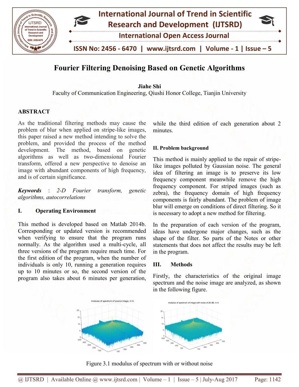
International Research Research and Development (IJTSRD) International Open Access Journal iltering Denoising Based on Genetic Algorithms iltering Denoising Based on Genetic Algorithms International Journal of Trend in Scientific Scientific (IJTSRD) International Open Access Journal ISSN No: 2456 ISSN No: 2456 - 6470 | www.ijtsrd.com | Volume 6470 | www.ijtsrd.com | Volume - 1 | Issue – 5 Fourier Filtering Denoising Based on Genetic Algorithms Jiahe Shi Faculty of Communication Engineering, Qiushi H Faculty of Communication Engineering, Qiushi Honor College, Tianjin University onor College, Tianjin University ABSTRACT As the traditional filtering methods may cause the problem of blur when applied on stripe this paper raised a new method intending to solve the problem, and provided the process of the method development. The method, based on genetic algorithms as well as two-dimensional Fourier transform, offered a new perspective to denoise an image with abundant components of high frequency, and is of certain significance. Keywords : 2-D Fourier algorithms, autocorrelations I. Operating Environment This method is developed based on Matlab 2014b. Corresponding or updated version is r when verifying to ensure that the program runs normally. As the algorithm used a multi three versions of the program require much time. For the first edition of the program, when the number of individuals is only 10, running a generat up to 10 minutes or so, the second version of the program also takes about 6 minutes per generation, As the traditional filtering methods may cause the problem of blur when applied on stripe-like images, this paper raised a new method intending to solve the problem, and provided the process of the method development. The method, based on genetic while the third edition of each generation about 2 while the third edition of each generation about 2 minutes. II. Problem background dimensional Fourier This method is mainly applied to the repair of stripe like images polluted by Gaussian noise. idea of filtering an image is to preserve its low frequency component meanwhile remove the high frequency component. For striped images (such as zebra), the frequency domain of high frequency components is fairly abundant. The problem of imag blur will emerge on conditions of direct filtering. So it is necessary to adopt a new method for filtering. is necessary to adopt a new method for filtering. This method is mainly applied to the repair of stripe- ages polluted by Gaussian noise. The general filtering an image is to preserve its low frequency component meanwhile remove the high frequency component. For striped images (such as zebra), the frequency domain of high frequency components is fairly abundant. The problem of image blur will emerge on conditions of direct filtering. So it transform, offered a new perspective to denoise an ith abundant components of high frequency, D Fourier transform, transform, genetic genetic This method is developed based on Matlab 2014b. Corresponding or updated version is recommended when verifying to ensure that the program runs normally. As the algorithm used a multi-cycle, all three versions of the program require much time. For the first edition of the program, when the number of individuals is only 10, running a generation requires up to 10 minutes or so, the second version of the program also takes about 6 minutes per generation, In the preparation of each version of the program, ideas have undergone major changes, such as the shape of the filter. So parts of the Notes or other statements that does not affect the results may be left In the preparation of each version of the program, ideas have undergone major changes, such as the shape of the filter. So parts of the Notes statements that does not affect the results may be left in the program. III. Methods Firstly, the characteristics of the original image spectrum and the noise image are analyzed, as shown Firstly, the characteristics of the original image spectrum and the noise image are analyzed, as shown in the following figure. Figure 3.1 modulus of spectrum with or without noise Figure 3.1 modulus of spectrum with or without noise @ IJTSRD | Available Online @ www.ijtsrd.com RD | Available Online @ www.ijtsrd.com | Volume – 1 | Issue – 5 | July-Aug 2017 Aug 2017 Page: 1142
International Journal of Trend in Scientific Research and Development (IJTSRD) ISSN: 2456 An image of zebra is used here. From the nature of the Fourier transform we know that the spectrum of the noise image is equal to the simple superposition of the noise spectrum and the image spectrum, i.e. nd the image spectrum, i.e. International Journal of Trend in Scientific Research and Development (IJTSRD) ISSN: 2456 An image of zebra is used here. From the nature of the Fourier transform we know that the spectrum of the noise image is equal to the simple superposition of the International Journal of Trend in Scientific Research and Development (IJTSRD) ISSN: 2456-6470 frequency component, it is also required a gradually transition from ellipse to circle as the major axis rameters of the filter, i.e., the direction of the ellipse, the initial eccentricity, the velocity of the transition to the circle, the trend of the attenuation value, are used as the genes in the genetic algorithm, and the optimal value is given by the frequency component, it is also required a gradually transition from ellipse to circle as the major axis increases. The parameters of the filter, i.e., the direction of the ellipse, the initial eccentricity, the velocity of the transition to the circle, the trend of the attenuation value, are used as the genes in the genetic algorithm, and the optimal value is given by the genetic algorithm. F F F ( ( A+n A +n ) ) ( ) A ( ) A ( ); n ( ); n Thus, the noise spectrum "submerges" the spectrum of the image. Since the noise spectrum is random and unpredictable, we cannot completely restore the image spectrum in the frequency domain when the noise spectrum is unknown, but only have the result spectrum approached as close as possible to the spectrum of the original image. This is the general idea of this method. From the above graphs we can see that the high-frequency part of the original image is obviously subsided, and after the noise is added, the high-frequency region is obviously uplifted and relatively flat. In the low frequency part, the original image spectrum "terrain" is higher, making the "submerged" effect of noise not significant. Namely there is no obvious difference in the trend in the low frequency part. Therefore, it is desirable to find a filter function that best fits the image through a genetic algorithm so that it can properly restore the trend of the spectrum. Thus, the noise spectrum "submerges" the spectrum of the image. Since the noise spectrum is random and unpredictable, we cannot completely restore the e frequency domain when the noise spectrum is unknown, but only have the result spectrum approached as close as possible to the spectrum of the original image. This is the general this method. From the above graphs we can ncy part of the original image is obviously subsided, and after the noise is added, the frequency region is obviously uplifted and relatively flat. In the low frequency part, the original image spectrum "terrain" is higher, making the ct of noise not significant. Namely there is no obvious difference in the trend in the low frequency part. Therefore, it is desirable to find a filter function that best fits the image through a genetic algorithm so that it can properly restore the Figure 3.3 example filter Figure 3.3 example filter The following figure shows the spectrum of the image flattened: The following figure shows the spectrum of the image In particular, taking the characteristics of abounding high frequency components of the fringe image into account, it is supposed to restore the high frequency details as much as possible under the prerequisite of ensuring that the image spectrum trend approaches that of the original image. For the question of how to extract the details of high frequency components from the noise image, the radient information and In particular, taking the characteristics of abounding high frequency components of the fringe image into account, it is supposed to restore the high frequency part of the spectral details as much as possible under the prerequisite of ensuring that the image spectrum trend approaches that of the original image. For the question of how to extract the details of high frequency components from the noise image, the method of obtaining gradient information and denoising with threshold is adopted in this method. denoising with threshold is adopted in this method. The gradient method is applied to extract the edge information of the image, that is, the high frequency component of the image. In this method, the gradient rivative (the difference) of the two , is calculated first, giving the direction of the most grayscale change at each point. ectional derivative (difference) is obtained then for this direction, so that the edge information of the image can be obtained. When the image is added Noise, the image edge information is obtained as The gradient method is applied to extract the edge information of the image, that is, the high frequency component of the image. In this method, the gradient of the image, the derivative (the difference) of the two directions x and y, is calculated first, giving the direction of the most grayscale change at each point. The directional derivative (difference) is obtained then for this direction, so that the edge information of the image can be obtained. When the image is added 20dB Noise, the image edge information is obtained as follows: Figure 3.2 modulus of spectrum of source image, in ln Figure 3.2 modulus of spectrum of source image, in ln In order to make the algorithm be generic, considering the characteristics of the image spectrum, the filter is set to a series of concentric ellipses. In order to obtain similar attenuation of the four corners of the high similar attenuation of the four corners of the high In order to make the algorithm be generic, considering pectrum, the filter is set to a series of concentric ellipses. In order to obtain @ IJTSRD | Available Online @ www.ijtsrd.com RD | Available Online @ www.ijtsrd.com | Volume – 1 | Issue – 5 | July-Aug 2017 Aug 2017 Page: 1143
International Journal of Trend in Scientific Research and Development (IJTSRD) ISSN: 2456 International Journal of Trend in Scientific Research and Development (IJTSRD) ISSN: 2456 International Journal of Trend in Scientific Research and Development (IJTSRD) ISSN: 2456-6470 It can be seen that although the edge of the image is also lost in some degree, it still retains part of the edge information. With this part of the edge information (rather than nothing at all), it will be possible to modify the high-frequency spectrum, and thus maximize the restoration of the details of the image. maximize the restoration of the details of the image. be seen that although the edge of the image is also lost in some degree, it still retains part of the edge information. With this part of the edge information (rather than nothing at all), it will be possible to frequency spectrum, and thus try to In the process of designing this method, there are three editions of program formed. The core idea of the three editions is to use genetic algorithm to achieve the optimal individual of filtering effect through several iterations. For genetic algorithms, there must be indicators that can be used to quantify the . And the main difference among the three editions of the program is that the indicator is selected different. The versions are In the process of designing this method, there are three editions of program formed. three editions is to use genetic algorithm to achieve the optimal individual of filtering effect through several iterations. For genetic algorithms, there must be indicators that can be used to quantify the restoration of individuals. And the main difference among the three editions of the program is that the indicator is selected different. The versions are described here separately. Figure 3.4 example of edge information Figure 3.4 example of edge information In order to restore as much as possible the noise high-frequency components from the information, considering that the magnitude of "edge information" formed by the noise tends to be low, a threshold is set thusly, ignoring the “edge information” where the gray value is less than the threshold. The process effect is as follows: In order to restore as much as possible the noise-free frequency components from the information, considering that the magnitude of "edge information" tends to be low, a threshold is set thusly, ignoring the “edge information” where the gray value is less than the threshold. The process 3.1 The first edition of the program 3.1 The first edition of the program The evaluation indicator of the first edition of the is the sharpness of the central peak of the autocorrelation function of the whole image. The The evaluation indicator of the first edition of the program is the sharpness of the central peak of the autocorrelation function of the whole image. The following demonstrates its principles. following demonstrates its principles. First the concept of two-dimensional autocorrelation function is explained. For m n m n dimensional autocorrelation order matrix: a a a a 11 11 1 1 n a a a a A = = ; ; ij ij in in a a a a a a m m 1 mj mj mn mn Define its cyclic shift as: Define its cyclic shift as: Figure 3.5 filtered edge information with threshold = 0.36 Figure 3.5 filtered edge information with threshold = 0.36 a a a a a a a a a a a a m p m p m p n q n q n q m p m p a a 1 a m p a m p a a 11 a m p m p a m p m p m p n q n q n q ( ( ( 1)( 1)( 1)( 1) 1) 1) ( ( ( 1) 1) 1) n n n ( ( ( 1)1 1)1 1)1 ( ( ( 1)( 1)( 1)( ) ) ) a a a a a a a a a a a a m n q a n q a n q a m n q m n q ( ( ( 1) 1) 1) mn mn mn m m m 1 1 1 m n q a m n q m n q ( ( ( ) ) ) A = = = ; ; ; n q n q n q n q 1( 1( 1( 1) 1) 1) 1 1 n n n 11 11 1( 1( 1( ) ) ) a a a a a a a a a a a a m p n q m p n q m p n q m p n m p n m p n m p m p m p m p n q m p n q m p n q ( ( ( )( )( )( 1) 1) 1) ( ( ( ) ) ) ( ( ( )1 )1 )1 ( ( ( )( )( )( ) ) ) @ IJTSRD | Available Online @ www.ijtsrd.com RD | Available Online @ www.ijtsrd.com | Volume – 1 | Issue – 5 | July-Aug 2017 Aug 2017 Page: 1144
International Journal of Trend in Scientific Research and Development (IJTSRD) ISSN: 2456 Referred to as pq A . Obviously, the fol expression is true forp and q: International Journal of Trend in Scientific Research and Development (IJTSRD) ISSN: 2456-6470 International Journal of Trend in Scientific Research and Development (IJTSRD) ISSN: 2456 . Obviously, the following p q m n ; Then the elements within its autocorrelation matrix can be given by the following equation: Then the elements within its autocorrelation matrix 1 R A A ; ; pq pq mn Where the symbol " " represents the dot product operation for the matrix, that is, the sum after the multiplication of the corresponding term. We can see that the above equation is actually an average value. For convenience, the autocorrelation matrix is expressed as: " represents the dot product operation for the matrix, that is, the sum after the multiplication of the corresponding term. We can see ove equation is actually an average value. For convenience, the autocorrelation matrix is Figure 3.1.2 R of the example image Figure 3.1.2 R of the example image So the filtering effect can be evaluated by judging the So the filtering effect can be evaluated by judging the sharpness of the matrix R . next step is to prove that the autocorrelation matrix of superposition of the image matrix A and equivalent in shape to the simple The next step is to prove that the autocorrelation matrix of superposition of the image matrix noise n is equivalent in shape to the simple superposition of the two autocorrelation matrices, i.e. position of the two autocorrelation matrices, i.e. R E ( A A ); (Equation 3.1.1) (Equation 3.1.1) A pq For white noise, that is, Gaussian noise, we know that its autocorrelation characteristics are very sharp, the value of the center peak is very large, whereas the non-center value is very small, as shown below: center value is very small, as shown below: For white noise, that is, Gaussian noise, we know that ation characteristics are very sharp, the value of the center peak is very large, whereas the R R = R +R + = R +R + C ; A+n A+n A A n n Available from Equation 3.1.1: Available from Equation 3.1.1: R R E E E (( (( (( (( ( ( A+n A+n A A A A A+n A+n ) ( ) ( pq ) ( ) ( A+n A n n n n A+n A ) ) pq +n ) ) +n A+n )) )) pq pq pq A n A n pq n A n A ) ) pq pq pq pq pq pq pq Note that the image matrix and noise should be Note that the image matrix and noise should be completely independent, so there are: pendent, so there are: E E ( ( n A n A ) ) E E ( ( n n A A ) ) E E ( ) n ( ) n E E ( ) A ( ) A C C ; ; pq pq In this way, the autocorrelation matrix of the image matrix with noise is equal to the autocorrelation matrix of the original autocorrelation matrix of the noise is superimposed as well as the whole lifted by the height of constant C . Thus the shape is equal to the simple superposition of In this way, the autocorrelation matrix of the image matrix with noise is equal to the autocorrelation matrix of the original autocorrelation matrix of the nois well as the whole lifted by the height of constant Thus the shape is equal to the simple superposition of both. image, image, where where the the Figure 3.1.1 R of matrix of 25dB white gauss noise Figure 3.1.1 R of matrix of 25dB white gauss noise For the general image, the autocorrelation matrix is relatively gentle, as shown in the following figure: relatively gentle, as shown in the following figure: orrelation matrix is In order to describe the sharpness of the spikes, also take the gradient method to obtain the maximum value of the directional derivative in the direction of gradient in the matrixR . And then the ratio of it to the average difference degree (i.e., standard deviation) of matrix R is used as a basis for measuring the sharpness of the spikes, which is: sharpness of the spikes, which is: In order to describe the sharpness of the spikes, also radient method to obtain the maximum value of the directional derivative in the direction of . And then the ratio of it to the average difference degree (i.e., standard deviation) of is used as a basis for measuring the @ IJTSRD | Available Online @ www.ijtsrd.com RD | Available Online @ www.ijtsrd.com | Volume – 1 | Issue – 5 | July-Aug 2017 Aug 2017 Page: 1145
International Journal of Trend in Scientific Research and Development (IJTSRD) ISSN: 2456-6470 max( ); R eliminating autocorrelation operation. the need for time-consuming R In fact, this version of the program has an erroneous principle. Since the filter is generated on the basis of the unknown contamination of the image, the filter generation statement cannot distinguish ( ( ) E A S , but only blindly pursue the minimum of ( ) E A+n S , leading ingredients of suffer a lot of losses. There is no way to solve this problem. The lower the ratio, the better the filtering effect. In the genetic algorithm thusly this ratio can act as an evaluation function, ascending order. E S ) versus n 3.2 The second edition of the program E ( S ) will also Although the first version of the program is theoretically feasible, but in practice due to the autocorrelation function call for too much time, another alternative evaluation indicators is required as substitute. The second edition of the program therefore takes the mean of power spectrum as the evaluation index. A 3.3 The third edition of the program The first two versions of the program is mainly aiming at finding a filter for the image through the analysis of the image, in order to achieve optimal filtering. Although theoretically feasible, the results of the operation of the filtering effect is very poor, and takes much time. In this context, the third version of the program's aim has undergone great changes. The third edition of the program tries to find a filter that is relatively effective for all images through sample training. In order to make the filter have generality, as well as to compress required time for the program, a completely concentric model is adopted instead of the ellipse-to-round transition filter model. Since it is a sample training, the evaluation indicator can be performed under conditions where free noise images are already available. Therefore, the mean square error of the filtered image and the original image is used as the evaluation indicator: From the Wiener-Khinchin theorem we know that the power spectrum and the autocorrelation function are a pair of Fourier transforms, i.e. F S ( ); R So we can get the power spectrum of the noise image: F F S ( ( R R ) A+n A+n R C) A S n S A n If we ignore the central impact, we can see that the power spectrum of the noise image is the superposition of the power spectrum of the original image and the noise image. So there is: m n 2 ' A A F E ( S ) E E ( ( ( S R )) ( S ij ij A+n A+n i 1 j 1 MSE ; ) E ) mn A n And because of: IV. Results of the operation 2 F S ( A +n ) ; 4.1 The first edition of the program A+n The following figure is the result of the first version of the program with the number of individual population set of 10, generations of 40, mutation rate of 0.1, noise of 25dB. The program requires 71.2 minutes. There must be a non-negative expected value of the power spectrum. So ( E A+n S evaluation indicator. The lower value of the indicator indicates more ingredients of image, i.e. better filtering effect. In this way, only the procedure of having the already calculated elements of the spectrum squared and averaged is needed, ) can be regardedas the E ( S ) filtered in the n @ IJTSRD | Available Online @ www.ijtsrd.com | Volume – 1 | Issue – 5 | July-Aug 2017 Page: 1146
International Journal of Trend in Scientific Research and Development (IJTSRD) ISSN: 2456-6470 Figure 4.1 result of the first edition of the program 4.2 The second edition of the program The following figure is the result of the second version of the program with the number of individual population set of 10, generations of 40, mutation rate of 0.1, noise of 25dB. The program requires 48.4 minutes. Figure 4.2 result of the second edition of the program 4.3 The third edition of the program The following figure is the result of the third version of the program with the number of individual population set of 10, generations of 40, mutation rate of 0.1, noise of 25dB . The program requires 6 minutes. @ IJTSRD | Available Online @ www.ijtsrd.com | Volume – 1 | Issue – 5 | July-Aug 2017 Page: 1147
International Journal of Trend in Scientific Research and Development (IJTSRD) ISSN: 2456-6470 Figure 4.3 result of the third edition of the program Although the problem of Gaussian denoising of high frequency image remained unsolved, this paper presents a new idea, which has certain significance. V Results and discussion As can be seen from the results of the operation, all of the three editions of the program cannot get satisfying results through genetic algorithm. One possible reason is that because of the limited time, parameter of individual number is set too small, resulting in the case where genetic algorithm quickly converge to the local solution. On the other hand, the selection of the indicator in genetic algorithm selection may not be scientific. In operation, it is found that genetic algorithms tend to screen out individuals whose edge information is completely erased. This shows scientific suspicion of the measure to use the unstandardized gradient edge information as the replacement of high-frequency component. VI Appendix: Program code 6.1 The first edition of the program %% %initializing clc; disp('GA image filtering version 1.0'); disp(' '); disp('Initializing...'); Another point that can be further improved is the denoising of the edge information. The current simple threshold method will cause a lot of losses of edge information. My initial idea is to use the Hog algorithm, that is, to find the gradient of each point in the image. We can see that the edge of the noise is often expressed as a scatter without continuity, and the edge direction of the real image is within a certain range consistent with the direction of the adjacent edge. Therefore, we can use the method of "moving hood" in median filter measure to analyze the gradient direction in a small area, so as to realize the filtering of noise. clear; close all; %% %reading the target image disp('Loading raw image...'); source = double(imread('zebra/Zebra.png')); [XD,YD] = size(source); @ IJTSRD | Available Online @ www.ijtsrd.com | Volume – 1 | Issue – 5 | July-Aug 2017 Page: 1148
International Journal of Trend in Scientific Research and Development (IJTSRD) ISSN: 2456-6470 max_r = sqrt((XD/2)^2 +(YD/2)^2); dB = input('What intensity of noise are you expecting?: '); %max_S = XD*YD/4; noise = wgn(XD, YD, dB); %% test = double(source) +noise; %loading parameters cal_t = fftshift(fft2(test)); disp(' '); angle_t = exp(1i*angle(cal_t)); disp('Loading parameters...'); show_t = log(1 +abs(cal_t)); generation = input('For how many generations are you expecting?: '); %overall generations of circulation in GA %% %extracting edge information while(generation <= 1 || mod(generation, 1) ~= 0) disp('Extracting edge information...'); disp('The parameter is supposed to be a positive integer greater than 1'); [TestX,TestY]=gradient(test); bevel_t = sqrt(TestX.^2+TestY.^2); generation = input('Please re-input the parameter: '); grad_t=TestX.*(TestX./bevel_t)+TestY.*(TestY./bev el_t); end grad_t(isnan(grad_t)) = 0; number = input('How many individuals are there in the flock?: '); %number of individual clear bevel_t TestX TestY; while(number <= 0 || mod(number, 2) ~= 0) %% disp('The parameter is supposed to be a positive even number'); %GA preparation disp(' '); number = input('Please re-input the parameter: '); disp('Initialization accomplished, preparing for the GA circulation...'); end mutate = input('What is the probability of mutation supposed to be?: '); %probability of mutating filter = ones(size(source)); %the contour elipses are specified by the following equation: while(mutate <= 0 || mutate >= 1) disp('The parameter is supposed to be located between 0 & 1'); % (1 -c*cos^2(theta))*x^2 +(1 -c*sin^2(theta))*y^2 +c*sin(2*theta)*x*y = constant mutate = input('Please re-input the parameter: '); %the filter function is as following: end % h(x) = x^4 +para_1*x^2 %% %h(x) ensures value at the center of the filter equals to 0, which will contrbute to the normalization procession. %adding noise disp(' '); para = [0.7, pi/3, -1, -10, 1, 0.36, 0.7]; disp('Adding noise...'); %the vector of parameter is sequenced as the following order: @ IJTSRD | Available Online @ www.ijtsrd.com | Volume – 1 | Issue – 5 | July-Aug 2017 Page: 1149
International Journal of Trend in Scientific Research and Development (IJTSRD) ISSN: 2456-6470 % [para_e, para_theta, para_velocity, para_2, para_1, para_range, para_threshold] grad_r(isnan(grad_r)) = 0; primitive_mark = max(grad_r(:))/std(grad_r(:)); %where para_range indicates the range of the filter's value, para_threshold restricts the threshold for the matrix grad to be set to zero, as well as para_velocity indicates the speed from a elipse to transform to a circle R = repmat(R, 1, 1, 2*number); mark = primitive_mark*ones(1, 2*number); clear primitive_mark R_estimated limits = [0, 0.9999; disp('Preparation accomplished, Launching the GA circulation...'); 0, pi; disp(' '); -1, 0; figure('Menubar','none','Name','Result Monitor','NumberTitle','off'); -10, -2; 0, 1; set(gcf, 'position', [239, 344, 1083, 420]); 0, 1; subplot(1, 2, 1); 0, 1]; handle_image = imshow(result(:, :, 1), []); limits_range = limits(:, 2) -limits(:, 1); title('Filtering Result'); %the limits of values of the paras are as follows: subplot(2, 2, 2); % para_e para_theta para_velocity para_1 para_range para_threshold para_coef handle_window = gca; area(best_mark, 'EdgeColor', [77/255, 144/255, 21/255], 'FaceColor', [49/255, 171/255, 118/255], 'YDataSource', 'best_mark'); % [0, 1) [0, pi) [-1, 0] [-10, -2] [0,1] [0, 1] [0, 1] index = ones(1, 2*number); hold on; para = repmat(para', 1, 2*number); plot(best_mark, 'x', 'Color', [249/255, 71/255, 71/255], 'YDataSource', 'best_mark', 'LineWidth', 1); best_mark = nan(1, generation); hold off; mark_range = [0, 1]; grid on; filter = repmat(filter, 1, 1, 2*number); axis([1, generation, mark_range(1), mark_range(2)]); result = repmat(test, 1, 1, 2*number); title('Trend of Best Score among Generations'); show_f = repmat(show_t, 1, 1, 2*number); xlabel('Generations'); R = xcorr2(test); ylabel('Marks'); R = R./std(R(:)); subplot(2, 6, 10); R_range = [min(min(R(:))), max(max(R(:)))]; colormap(gca, parula); [DiffX, DiffY] = gradient(R); surf(filter(:, :, 1), 'ZDataSource', 'filter(:, :, 1)'); bevel_r = sqrt(DiffX.^2 +DiffY.^2); shading interp; grad_r +DiffY.*(DiffY./bevel_r); = DiffX.*(DiffX./bevel_r) @ IJTSRD | Available Online @ www.ijtsrd.com | Volume – 1 | Issue – 5 | July-Aug 2017 Page: 1150
International Journal of Trend in Scientific Research and Development (IJTSRD) ISSN: 2456-6470 alpha(0.7); %% xlim([1, XD]); %GA circulation ylim([1, YD]); disp('Starting the first generation...'); zlim([0, 1]); tic; set(gca, 'xtick', [], 'xticklabel', []); for t = 1 : generation set(gca, 'ytick', [], 'yticklabel', []); %generating new population camproj('perspective'); couple = randperm(number); %free mating title('Filter'); for i = 1 : 2 : number subplot(2, 6, 11); for node = 1 : size(para, 1) colormap(gca, parula); %swap genes mesh(show_f(:, :, 1), 'ZDataSource', 'show_f(:, :, 1)'); if(round(rand)) para(node, i +number) = para(node, i); xlim([1, XD]); para(node, i +number +1) = para(node, i +1); ylim([1, YD]); else zlim([min(show_t(:)), max(show_t(:))]); para(node, i +number) = para(node, i +1); set(gca, 'xtick', [], 'xticklabel', []); para(node, i +number +1) = para(node, i); set(gca, 'ytick', [], 'yticklabel', []); end camproj('perspective'); %mutation title('Spectrum'); if(rand < mutate) subplot(2, 6, 12); para(node, i +number) = limits(node, 1) +limits_range(node)*rand; colormap(gca, parula); contour3(R(:, :, 1), 30,'ZDataSource', 'R(:, :, 1)'); end box off; if(rand < mutate) para(node, i +number +1) = limits(node, 1) +limits_range(node)*rand; xlim([1, size(R, 1)]); ylim([1, size(R, 2)]); end zlim(R_range); end set(gca, 'xtick', [], 'xticklabel', []); clear node set(gca, 'ytick', [], 'yticklabel', []); end camproj('perspective'); clear i; title('Autocorrelation'); %characterizing individuals drawnow; @ IJTSRD | Available Online @ www.ijtsrd.com | Volume – 1 | Issue – 5 | July-Aug 2017 Page: 1151
International Journal of Trend in Scientific Research and Development (IJTSRD) ISSN: 2456-6470 for i = number +1 : 2*number %scoring %filter generating R(:, :, i) = xcorr2(result(:, :, i)); for j = 1 : XD; R_temp = R(:, :, i); for k = 1 : YD; R(:, :, i) = R_temp./std(R_temp(:)); ellipse = (1 -para(1, i)*cos(para(2, i))^2)*(j - XD/2)^2 +(1 -para(1, i)*sin(para(2, i))^2)*(k - YD/2)^2 +para(1, i)*sin(2*para(2, i))*(j -XD/2)*(k - YD/2); [DiffX, DiffY] = gradient(R(:, :, i)); bevel_r = sqrt(DiffX.^2 +DiffY.^2); grad_r +DiffY.*(DiffY./bevel_r); = DiffX.*(DiffX./bevel_r) ellipse = pi*ellipse/sqrt(1 -(para(1, i)^2)); grad_r(isnan(grad_r)) = 0; circle = pi*((j -XD/2)^2 +(k -YD/2)^2); mark(i) = max(grad_r(:))/std(grad_r(:)); r = sqrt(circle/pi); end ratio = r/max_r; clear i; portion = para(3, i)*ratio^2 -(para(3, i) +1)*ratio +1; %natual selecting element portion)*circle)/(max_r)^2/pi; = (portion*ellipse +(1 - [mark, index] = sort(mark); para = para(:, index); filter(j, k, i) = element^2 +para(4, i)*element; filter = filter(:, :, index); end R = R(:, :, index); clear k; show_f = show_f(:, :, index); end result = result(:, :, index); clear j; best_mark(t) = mark(1); filter(:, :, i) = filter(:, :, i)/max(max(abs(filter(:, :, i))))*para(5, i) +1; %demonstrating champion %profile modifying mark_range = minmax(best_mark); grad_temp = grad_t; mark_range(1) = mark_range(1)*0.99; grad_temp(grad_temp +std(grad_temp(:)))*para(6, i)) = 0; < (max(grad_temp(:)) mark_range(2) = mark_range(2)/0.99; set(handle_image, 'CData', result(:, :, 1)); cal_h = fftshift(fft2(grad_temp)); set(handle_window, 'YLim', mark_range); show_h = para(7, i)*log(1 +abs(cal_h)); refreshdata; %filtering drawnow; show_f(:, :, i) = show_t.*filter(:, :, i) +show_h.*(1 - filter(:, :, i)); %informing disp(['Generation #',num2str(t),' has finished']); cal_f = (exp(show_f(:, :, i)) -1).*angle_t; toc; result(:, :, i) = abs(ifft2(fftshift(cal_f))); @ IJTSRD | Available Online @ www.ijtsrd.com | Volume – 1 | Issue – 5 | July-Aug 2017 Page: 1152
International Journal of Trend in Scientific Research and Development (IJTSRD) ISSN: 2456-6470 beep; %% disp(' '); %reading the target image %terminate circle disp('Loading raw image...'); if(t > 2) source = double(imread('zebra/Zebra.png')); if(best_mark(t) == best_mark(t -1) && best_mark(t -1) == best_mark(t -2)) [XD,YD] = size(source); max_r = sqrt((XD/2)^2 +(YD/2)^2); break; %% end %adding noise end disp(' '); end disp('Adding noise...'); %% dB = input('What intensity of noise are you expecting?: '); %display result figure('Menubar','none','Name','Result comparasion','NumberTitle','off'); while(isempty(dB)) dB = input('Waiting for input...'); set(gcf, 'position', [239, 162, 1083, 601]); end subplot(1, 2, 1); noise = wgn(XD, YD, dB); imshow(test, [min(test(:)), max(test(:))]); test = double(source) +noise; title('Input Image'); cal_t = fftshift(fft2(test)); subplot(1, 2, 2); angle_t = exp(1i*angle(cal_t)); imshow(result(:, :, 1), [min(test(:)), max(test(:))]); show_t = log(1 +abs(cal_t)); title('Filtering Result'); %% %clear ellipse a ratio portion element r circle square; %loading parameters 6.2 The second edition of the program disp(' '); %% disp('Loading parameters...'); %initializing generation = input('For how many generations are you expecting?: '); %overall generations of circulation in GA clc; disp('GA image filtering version 2.0'); while(generation <= 1 || mod(generation, 1) ~= 0) disp(' '); disp('The parameter is supposed to be a positive integer greater than 1'); disp('Initializing...'); clear; generation = input('Please re-input the parameter: '); close all; @ IJTSRD | Available Online @ www.ijtsrd.com | Volume – 1 | Issue – 5 | July-Aug 2017 Page: 1153
International Journal of Trend in Scientific Research and Development (IJTSRD) ISSN: 2456-6470 end %the filter function is as following: number = input('How many individuals are there in the flock?: '); %number of individual % h(x) = x^4 +para_1*x^2 %h(x) ensures value at the center of the filter equals to 0, which will contrbute to the normalization procession. while(number <= 0 || mod(number, 2) ~= 0) disp('The parameter is supposed to be a positive even number'); para = [0.7, pi/3, -1, -10, 1, 0.36, 0.7]; %the vector of parameter is sequenced as the following order: number = input('Please re-input the parameter: '); end % [para_e, para_theta, para_velocity, para_2, para_1, para_range, para_threshold] mutate = input('What is the probability of mutation supposed to be?: '); %probability of mutating %where para_range indicates the range of the filter's value, para_threshold restricts the threshold for the matrix grad to be set to zero, as well as para_velocity indicates the speed from a elipse to transform to a circle while(mutate <= 0 || mutate >= 1) disp('The parameter is supposed to be located between 0 & 1'); mutate = input('Please re-input the parameter: '); limits = [0, 0.9999; end 0, pi; %% -1, 0; %extracting edge information -10, -2; disp('Extracting edge information...'); 0, 1; [TestX,TestY]=gradient(test); 0, 1; bevel_t = sqrt(TestX.^2+TestY.^2); 0, 1]; grad_t=TestX.*(TestX./bevel_t)+TestY.*(TestY./bev el_t); limits_range = limits(:, 2) -limits(:, 1); %the limits of values of the paras are as follows: grad_t(isnan(grad_t)) = 0; % para_e para_theta para_velocity para_1 para_range para_threshold para_coef clear bevel_t TestX TestY; %% % [0, 1) [0, pi) [-1, 0] [-10, -2] [0,1] [0, 1] [0, 1] %GA preparation %para_coef has currently been removed disp(' '); index = ones(1, 2*number); disp('Initialization accomplished, preparing for the GA circulation...'); para = repmat(para', 1, 2*number); filter = ones(size(source)); best_mark = nan(1, generation); %the contour elipses are specified by the following equation: mark_range = [0, 1]; % (1 -c*cos^2(theta))*x^2 +(1 -c*sin^2(theta))*y^2 +c*sin(2*theta)*x*y = constant filter = repmat(filter, 1, 1, 2*number); @ IJTSRD | Available Online @ www.ijtsrd.com | Volume – 1 | Issue – 5 | July-Aug 2017 Page: 1154
International Journal of Trend in Scientific Research and Development (IJTSRD) ISSN: 2456-6470 result = repmat(test, 1, 1, 2*number); area(percentage, 'EdgeColor', 'none', 'FaceColor', [49/255, 171/255, 118/255], 'percentage'); 'YDataSource', show_f = repmat(show_t, 1, 1, 2*number); grad_show = repmat(grad_t, 1, 1, 2*number); set(gca, 'xtick', [], 'xticklabel', []); power = (abs(fftshift(fft2(test)))).^2; set(gca, 'ytick', [], 'yticklabel', []); primitive_mark = mean(power(:)); ylim([0, 1]); mark = primitive_mark*ones(1, 2*number); title('Progress'); percentage = [0, 0]; subplot(3, 5, 3); clear primitive_mark R_estimated colormap(gca, parula); disp('Preparation accomplished, Launching the GA circulation...'); surf(filter(:, :, 1), 'ZDataSource', 'filter(:, :, 1)'); shading interp; disp(' '); alpha(0.7); figure('Menubar','none','Name','Result Monitor','NumberTitle','off'); xlim([1, XD]); set(gcf, 'position', [237, 195, 1083, 650]); ylim([1, YD]); subplot(3, 5, [1, 2, 6, 7]); zlim([0, 1]); handle_image = imshow(result(:, :, 1), []); set(gca, 'xtick', [], 'xticklabel', []); title('Filtering Result'); set(gca, 'ytick', [], 'yticklabel', []); subplot(3, 11, 23:32); camproj('perspective'); handle_window = gca; title('Filter'); area(best_mark, 'EdgeColor', [77/255, 144/255, 21/255], 'FaceColor', [49/255, 171/255, 118/255], 'YDataSource', 'best_mark'); subplot(3, 5, 8); colormap(gca, parula); mesh(show_f(:, :, 1), 'ZDataSource', 'show_f(:, :, 1)'); hold on; plot(best_mark, 'x', 'Color', [249/255, 71/255, 71/255], 'YDataSource', 'best_mark', 'LineWidth', 1); xlim([1, XD]); ylim([1, YD]); hold off; zlim([min(show_t(:)), max(show_t(:))]); grid on; set(gca, 'xtick', [], 'xticklabel', []); axis([1, generation, mark_range(1), mark_range(2)]); set(gca, 'ytick', [], 'yticklabel', []); title('Trend of Best Score among Generations'); camproj('perspective'); xlabel('Generations'); title('Spectrum'); ylabel('Marks'); subplot(3, 5, [4, 5, 9, 10]); subplot(3, 11, 33); handle_grad = imshow(grad_show(:, :, 1), []); @ IJTSRD | Available Online @ www.ijtsrd.com | Volume – 1 | Issue – 5 | July-Aug 2017 Page: 1155
International Journal of Trend in Scientific Research and Development (IJTSRD) ISSN: 2456-6470 title('Edge Information'); end drawnow; clear i; %% %characterizing individuals %GA circulation for i = number +1 : 2*number percentage 1)/number;refreshdata;drawnow; = [1, 1]*(i -number - disp('Starting the first generation...'); tic; %filter generating for t = 1 : generation for j = 1 : XD; percentage = [0, 0];refreshdata;drawnow; for k = 1 : YD; %generating new population ellipse = (1 -para(1, i)*cos(para(2, i))^2)*(j - XD/2)^2 +(1 -para(1, i)*sin(para(2, i))^2)*(k - YD/2)^2 +para(1, i)*sin(2*para(2, i))*(j -XD/2)*(k - YD/2); couple = randperm(number); %free mating for i = 1 : 2 : number for node = 1 : size(para, 1) ellipse = pi*ellipse/sqrt(1 -(para(1, i)^2)); %swap genes circle = pi*((j -XD/2)^2 +(k -YD/2)^2); if(round(rand)) %square = ((max(abs(j -XD/2), abs(k - YD/2)))^2); para(node, i +number) = para(node, i); r = sqrt(circle/pi); para(node, i +number +1) = para(node, i +1); ratio = r/max_r; else %ratio = sqrt(square/max_S); para(node, i +number) = para(node, i +1); portion = para(3, i)*ratio^2 -(para(3, i) +1)*ratio +1; para(node, i +number +1) = para(node, i); end element portion)*circle)/(max_r)^2/pi; = (portion*ellipse +(1 - %mutation if(rand < mutate) %element = (portion*elipse/max_elipse +(1 - portion)*square/max_S); para(node, i +number) = limits(node, 1) +limits_range(node)*rand; filter(j, k, i) = element^2 +para(4, i)*element; end end if(rand < mutate) clear k; para(node, i +number +1) = limits(node, 1) +limits_range(node)*rand; end clear j; end filter(:, :, i) = filter(:, :, i)/max(max(abs(filter(:, :, i))))*para(5, i) +1; end clear node %profile modifying @ IJTSRD | Available Online @ www.ijtsrd.com | Volume – 1 | Issue – 5 | July-Aug 2017 Page: 1156
International Journal of Trend in Scientific Research and Development (IJTSRD) ISSN: 2456-6470 grad_temp = grad_t; refreshdata; grad_temp(grad_temp +std(grad_temp(:)))*para(6, i)) = 0; < (max(grad_temp(:)) drawnow; %informing grad_show(:, :, i) = grad_temp; disp(['Generation #',num2str(t),' has finished']); cal_h = fftshift(fft2(grad_temp)); toc; show_h = log(1 +abs(cal_h)); beep; %filtering disp(' '); show_f(:, :, i) = show_t.*filter(:, :, i) +show_h.*(1 - filter(:, :, i)); %terminate circle if(t > 2) cal_f = (exp(show_f(:, :, i)) -1).*angle_t; if(best_mark(t) == best_mark(t -1) && best_mark(t -1) == best_mark(t -2)) result(:, :, i) = abs(ifft2(fftshift(cal_f))); %scoring break; power = (abs(cal_f)).^2; end mark(i) = mean(power(:)); end end end clear i; %% %natual selecting %display result [mark, index] = sort(mark); disp('Circulation terminated'); para = para(:, index); figure('Menubar','none','Name','Result comparasion','NumberTitle','off'); filter = filter(:, :, index); grad_show = grad_show(:, :, index); set(gcf, 'position', [237, 195, 1083, 650]); show_f = show_f(:, :, index); subplot(1, 2, 1); result = result(:, :, index); imshow(test, [min(test(:)), max(test(:))]); best_mark(t) = mark(1); title('Input Image'); %demonstrating champion subplot(1, 2, 2); mark_range = minmax(best_mark); imshow(result(:, :, 1), [min(test(:)), max(test(:))]); mark_range(1) = mark_range(1)*0.99; title('Filtering Result'); mark_range(2) = mark_range(2)/0.99; %clear ellipse a ratio portion element r circle square; set(handle_image, 'CData', result(:, :, 1)); 6.3 The third edition of the program set(handle_grad, 'CData', grad_show(:, :, 1)); %% set(handle_window, 'YLim', mark_range); %initializing @ IJTSRD | Available Online @ www.ijtsrd.com | Volume – 1 | Issue – 5 | July-Aug 2017 Page: 1157
International Journal of Trend in Scientific Research and Development (IJTSRD) ISSN: 2456-6470 clc; %% disp('GA image filtering version 3.0'); %loading parameters disp(' '); disp(' '); disp('Initializing...'); disp('Loading parameters...'); generation = input('For how many generations are you expecting?: '); %overall generations of circulation in GA clear; close all; %% while(generation <= 1 || mod(generation, 1) ~= 0) %reading the target image disp('The parameter is supposed to be a positive integer greater than 1'); disp('Loading raw image...'); generation = input('Please re-input the parameter: '); source = double(imread('zebra/Zebra.png')); [XD,YD] = size(source); end disp('Loading training sample...'); number = input('How many individuals are there in the flock?: '); %number of individual test(:, 20_22.1947.png')); :, 1) = double(imread('zebra/ZebraG while(number <= 0 || mod(number, 2) ~= 0) test(:, 30_18.8633.png')); :, 2) = double(imread('zebra/ZebraG disp('The parameter is supposed to be a positive even number'); test(:, 40_16.5752.png')); :, 3) = double(imread('zebra/ZebraG number = input('Please re-input the parameter: '); end test(:, 50_14.8842.png')); :, 4) = double(imread('zebra/ZebraG mutate = input('What is the probability of mutation supposed to be?: '); %probability of mutating test(:, 60_13.5614.png')); :, 5) = double(imread('zebra/ZebraG while(mutate <= 0 || mutate >= 1) sample = size(test, 3) disp('The parameter is supposed to be located between 0 & 1'); cal_t = test; mutate = input('Please re-input the parameter: '); angle_t = test; end show_t = test; %% for i = 1 : sample; %extracting edge information cal_t(:, :, i) = fftshift(fft2(test(:, :, i))); disp(' '); angle_t(:, :, i) = exp(1i*angle(cal_t(:, :, i))); disp('Extracting edge information...'); show_t(:, :, i) = log(1 +abs(cal_t(:, :, i))); grad_t = test; end for i = 1 : sample; clear i; [TestX,TestY]=gradient(test(:, :, i)); @ IJTSRD | Available Online @ www.ijtsrd.com | Volume – 1 | Issue – 5 | July-Aug 2017 Page: 1158
International Journal of Trend in Scientific Research and Development (IJTSRD) ISSN: 2456-6470 bevel_t = sqrt(TestX.^2+TestY.^2); index = ones(1, 2*number); grad_t(:, i)=TestX.*(TestX./bevel_t)+TestY.*(TestY./bevel_t); :, para = repmat(para', 1, 2*number); best_mark = nan(1, generation); end mark_temp = zeros(1, sample); grad_t(isnan(grad_t)) = 0; mark_range = [0, 1]; clear bevel_t TestX TestY i; filter = repmat(filter, 1, 1, 2*number); %% result = repmat(test, 1, 1, 1, 2*number); %GA preparation show_f = repmat(show_t, 1, 1, 1, 2*number); disp(' '); grad_show = repmat(grad_t, 1, 1, 1, 2*number); disp('Initialization accomplished, preparing for the GA circulation...'); show_h = zeros(XD, YD, sample); for j = 1 : sample filter = ones(size(source)); diff_temp = result(:, :, j, 1) - source; %the filter function is as following: mark_temp(j) = std(diff_temp(:)); % h(x) = x^4 +para_1*x^2 end %h(x) ensures value at the center of the filter equals to 0, which will contrbute to the normalization procession. clear j; mark = mean(mark_temp)*ones(1, 2*number); para = [-10, 0.4, 0.36, 0.42]; percentage = [0, 0]; %the vector of parameter is sequenced as the following order: disp('Preparation accomplished, Launching the GA circulation...'); % para_threshold, para_coef] [para_velocity, para_1, para_range, disp(' '); %where para_range indicates the range of the filter's value, para_threshold restricts the threshold for the matrix grad to be set to zero, as well as para_velocity indicates the speed from a elipse to transform to a circle show_result = zeros(XD, YD); show_grad = zeros(XD, YD); f_show = zeros(XD, YD); for j = 1 : sample limits = [-10, 0; show_result = show_result + result(:, :, j, 1); 0, 1; show_grad = show_grad + grad_show(:, :, j, 1); 0, 1; f_show = f_show + show_f(:, :, j, 1); 0, 1]; end limits_range = limits(:, 2) -limits(:, 1); clear j; %the limits of values of the paras are as follows: show_result = show_result./sample; % para_1 para_range para_threshold para_coef show_grad = show_grad./sample; % [-10, -2] [0,1] [0, 1] [0, 1] @ IJTSRD | Available Online @ www.ijtsrd.com | Volume – 1 | Issue – 5 | July-Aug 2017 Page: 1159
International Journal of Trend in Scientific Research and Development (IJTSRD) ISSN: 2456-6470 f_show = f_show./sample; %box off; figure('Menubar','none','Name','Result Monitor','NumberTitle','off'); surf(filter(:, :, 1), 'ZDataSource', 'filter(:, :, 1)'); shading interp; set(gcf, 'position', [237, 195, 1083, 650]); alpha(0.7); subplot(3, 5, [1, 2, 6, 7]); xlim([1, XD]); handle_image = imshow(show_result, []); ylim([1, YD]); title('Filtering Result'); zlim([0, 1]); subplot(3, 11, 23:32); set(gca, 'xtick', [], 'xticklabel', []); handle_window = gca; set(gca, 'ytick', [], 'yticklabel', []); area(best_mark, 'EdgeColor', [77/255, 144/255, 21/255], 'FaceColor', [49/255, 171/255, 118/255], 'YDataSource', 'best_mark'); camproj('perspective'); title('Filter'); hold on; subplot(3, 5, 8); plot(best_mark, 'x', 'Color', [249/255, 71/255, 71/255], 'YDataSource', 'best_mark', 'LineWidth', 1); colormap(gca, parula); mesh(f_show, 'ZDataSource', 'f_show'); hold off; xlim([1, XD]); grid on; ylim([1, YD]); axis([1, generation, mark_range(1), mark_range(2)]); zlim([min(show_t(:)), max(show_t(:))]); title('Trend of Best Score among Generations'); set(gca, 'xtick', [], 'xticklabel', []); xlabel('Generations'); set(gca, 'ytick', [], 'yticklabel', []); ylabel('Marks'); camproj('perspective'); subplot(3, 11, 33); title('Spectrum'); area(percentage, 'EdgeColor', 'none', 'FaceColor', [49/255, 171/255, 118/255], 'percentage'); 'YDataSource', subplot(3, 5, [4, 5, 9, 10]); handle_grad = imshow(show_grad, []); set(gca, 'xtick', [], 'xticklabel', []); title('Edge Information'); set(gca, 'ytick', [], 'yticklabel', []); drawnow; ylim([0, 1]); %% title('Progress'); %GA circulation subplot(3, 5, 3); disp('Starting the first generation...'); colormap(gca, parula); tic; %contour3(filter(:, :, 1), 30, 'ZDataSource', 'filter(:, :, 1)'); for t = 1 : generation @ IJTSRD | Available Online @ www.ijtsrd.com | Volume – 1 | Issue – 5 | July-Aug 2017 Page: 1160
International Journal of Trend in Scientific Research and Development (IJTSRD) ISSN: 2456-6470 percentage = [0, 0];refreshdata;drawnow; filter(j, k, i) = -circle^2 +para(1, i)*circle; %generating new population end couple = randperm(number); %free mating end filter(:, :, i) = filter(:, :, i)/max(max(abs(filter(:, :, i))))*para(2, i) +1; for i = 1 : 2 : number for node = 1 : size(para, 1) %profile modifying %swap genes for j = 1 : sample if(round(rand)) grad_temp = grad_t(:, :, j); para(node, i +number) = para(node, i); grad_temp(grad_temp +std(grad_temp(:)))*para(3, i)) = 0; < (max(grad_temp(:)) para(node, i +number +1) = para(node, i +1); else grad_show(:, :, j, i) = grad_temp; para(node, i +number) = para(node, i +1); cal_h = fftshift(fft2(grad_temp)); para(node, i +number +1) = para(node, i); show_h(:, :, j) = log(1 +abs(cal_h)); end end %mutation %filtering if(rand < mutate) for j = 1 : sample para(node, i +number) = limits(node, 1) +limits_range(node)*rand; show_f(:, :, j, i) = show_t(:, :, j).*filter(:, :, i) +show_h(:, :, j).*(1 -filter(:, :, i)).*para(4, i); end cal_f = (exp(show_f(:, :, j, i)) -1).*angle_t(:, :, j); if(rand < mutate) result(:, :, j, i) = abs(ifft2(fftshift(cal_f))); para(node, i +number +1) = limits(node, 1) +limits_range(node)*rand; end %scoring end for j = 1 : sample end diff_temp = result(:, :, j, i) - source; end mark_temp(j) = std(diff_temp(:)); %characterizing individuals end for i = number +1 : 2*number mark(i) = mean(mark_temp); percentage number)/number;refreshdata;drawnow; = [1, 1]*(i - end %filter generating %natual selecting for j = 1 : XD; [mark, index] = sort(mark); for k = 1 : YD; para = para(:, index); circle = pi*((j -XD/2)^2 +(k -YD/2)^2); filter = filter(:, :, index); @ IJTSRD | Available Online @ www.ijtsrd.com | Volume – 1 | Issue – 5 | July-Aug 2017 Page: 1161
International Journal of Trend in Scientific Research and Development (IJTSRD) ISSN: 2456-6470 grad_show = grad_show(:, :, :, index); if(best_mark(t) == best_mark(t -1) && best_mark(t -1) == best_mark(t -2)) show_f = show_f(:, :, :, index); break; result = result(:, :, :, index); end best_mark(t) = mark(1); end %demonstrating champion end mark_range = minmax(best_mark); %% mark_range(1) = mark_range(1)*0.99; %display result mark_range(2) = mark_range(2)/0.99; disp('Circulation terminated'); show_result = zeros(XD, YD); figure('Menubar','none','Name','Result comparasion','NumberTitle','off'); show_grad = zeros(XD, YD); for j = 1 : sample set(gcf, 'position', [237, 195, 1083, 650]); show_result = show_result + result(:, :, j, 1); subplot(1, 2, 1); show_grad = show_grad + grad_show(:, :, j, 1); imshow(source, []); f_show = f_show + show_f(:, :, j, 1); title('Target Image'); end subplot(1, 2, 2); show_result = show_result./sample; imshow(show_result, []); show_grad = show_grad./sample; title('Filtering Result'); f_show = f_show./sample; %clear ellipse a ratio portion element r circle square; set(handle_image, 'CData', show_result); set(handle_grad, 'CData', show_grad); set(handle_window, 'YLim', mark_range); refreshdata; drawnow; %informing disp(['Generation #',num2str(t),' has finished']); toc; beep; disp(' '); %terminate circle if(t > 2) @ IJTSRD | Available Online @ www.ijtsrd.com | Volume – 1 | Issue – 5 | July-Aug 2017 Page: 1162