Download
1 / 8
80 likes | 91 Views
In this paper, we design controller that combines an observer and a control to handle systems subject to actuator or sensor degradation including complete failure . The observer contains a pre filter, an adaptive law, and a modified Luenberger observer that achieves estimation of system state and estimation of conditions of actuator or sensor. We have shown that if a set of differential Riccati inequatities DRI is satisfied then the system can be stabilized under actuator degrad ation. While in sensor degradation case if an Algebraci Riccati inequality ARI and a DRI are satisfied then the system is stabilized. Chieh-Chuan Feng "Control Systems in the Presence of Actuators or Sensors Degradation" Published in International Journal of Trend in Scientific Research and Development (ijtsrd), ISSN: 2456-6470, Volume-1 | Issue-5 , August 2017, URL: https://www.ijtsrd.com/papers/ijtsrd2250.pdf Paper URL: http://www.ijtsrd.com/engineering/electrical-engineering/2250/control-systems-in-the-presence-of-actuators-or-sensors-degradation/chieh-chuan-feng<br>

E N D
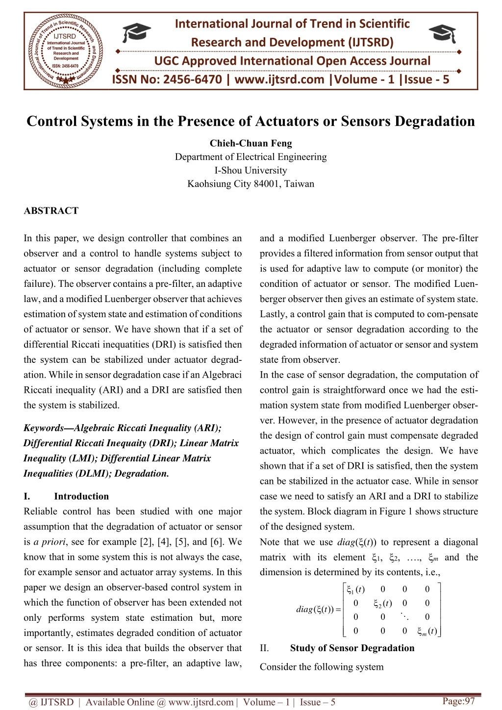
International Journal of Trend in Scientific Research and Development (IJTSRD) UGC Approved International Open Access Journal ISSN No: 2456‐6470 | www.ijtsrd.com |Volume ‐ 1 |Issue ‐ 5 Control Systems in the Presence of Actuators or Sensors Degradation Chieh-Chuan Feng Department of Electrical Engineering I-Shou University Kaohsiung City 84001, Taiwan ABSTRACT In this paper, we design controller that combines an observer and a control to handle systems subject to actuator or sensor degradation (including complete failure). The observer contains a pre-filter, an adaptive law, and a modified Luenberger observer that achieves estimation of system state and estimation of conditions of actuator or sensor. We have shown that if a set of differential Riccati inequatities (DRI) is satisfied then the system can be stabilized under actuator degrad- ation. While in sensor degradation case if an Algebraci Riccati inequality (ARI) and a DRI are satisfied then the system is stabilized. and a modified Luenberger observer. The pre-filter provides a filtered information from sensor output that is used for adaptive law to compute (or monitor) the condition of actuator or sensor. The modified Luen- berger observer then gives an estimate of system state. Lastly, a control gain that is computed to com-pensate the actuator or sensor degradation according to the degraded information of actuator or sensor and system state from observer. In the case of sensor degradation, the computation of control gain is straightforward once we had the esti- mation system state from modified Luenberger obser- ver. However, in the presence of actuator degradation the design of control gain must compensate degraded actuator, which complicates the design. We have shown that if a set of DRI is satisfied, then the system can be stabilized in the actuator case. While in sensor case we need to satisfy an ARI and a DRI to stabilize the system. Block diagram in Figure 1 shows structure of the designed system. Note that we use diag((t)) to represent a diagonal matrix with its element 1, 2, …., m and the dimension is determined by its contents, i.e., 0 )) ( ( t diag Keywords—Algebraic Riccati Inequality (ARI); Differential Riccati Inequaity (DRI); Linear Matrix Inequality (LMI); Differential Linear Matrix Inequalities (DLMI); Degradation. I. Reliable control has been studied with one major assumption that the degradation of actuator or sensor is a priori, see for example [2], [4], [5], and [6]. We know that in some system this is not always the case, for example sensor and actuator array systems. In this paper we design an observer-based control system in which the function of observer has been extended not only performs system state estimation but, more importantly, estimates degraded condition of actuator or sensor. It is this idea that builds the observer that has three components: a pre-filter, an adaptive law, Introduction t ( ) 0 0 0 1 t ( ) 0 0 2 0 0 0 t 0 0 0 ( ) m II. Study of Sensor Degradation Consider the following system Page:97 @ IJTSRD | Available Online @ www.ijtsrd.com | Volume – 1 | Issue – 5
International Journal of Trend in Scientific Research and Development(IJTSRD) ISSN: 2456-6470 The properties addressed above have the following interpretations: (1)k(t) = 0 means the actuator fails. k(t) = 1 means the actuator works properly. A degraded actuator will be 0 < k(t) < 1. x t Ax t Bu t ( ) ( ) ( ) y t Cx t ( ) t ( ) (1) y diag t y t ( ) ( ( )) ( ) s where the x(t) Rn represents the control input, y(t) Rv is the system output, and ys(t)Rv is the true signal output of the system from sensors. The diagonal element of diag((t)), k(t) R, k = 1, ..., v, is to represent the remaining function of the associated sensor. For example, if an sensor k = 0.80, then we say the sensor has 80% functioning. u(t)Rm is the control signals that will be fed into the actuators with observed state ( ) ( ˆ t x ) as the feedback signals, i.e. ti ( t ) means that the degradation is a k lim t 0 0 piecewise constant process. Under the process we allow k(t) to have jumps toward zero. We now state the observer and controller problem for the sensor degradation case as follows. Problem 1 Consider the system (1) with controller (2) and observer(3). Find, if possible, the controller and observer which comprises of a pre-filter, an ( ˆ x u t K t ( ) ) (2) with K the feedback gain. adaptive law for ( ) t , and a state observer of ( ˆ t x ) Controller gain with gain L such that Plant Sensors Actuators (A)( ) t is an estimate of (t) and ( ) Feedback signals t ( ) t is Pre-filter Adaptive law State observer bounded (which will always be the case if Observer ˆ t t for all k = 1, …, 0 ( ) 1 since 0 ( ) 1 Figure 1 Block diagram of system structure k k v). We now consider a state observer of following form: ( ˆ t x ( ˆ ( (B) converges to x(t), i.e. . x t x t ) lim t ) ( )) 0 (ˆ( ( ˆ x ( ˆ x ( ˆ x t A t Bu t L y t diag t C t ) ) ( ) ( ( ) )) )) s (3) (C)The state observer is asymptotically stable. (D)The controller ( t u closed-loop system with observer achieving (A), (B), and (C) is asymptotically stable. ( ˆ y ( ˆ x t C t ) ) ( ˆ x K t is such that the ) ) Rn is the state of observer, L is the ( ˆ t x where observer gain to be designed, ( ) estimation of y(t) and the true sensor output ys(t) is ) y tRv is an Theorem 2 Problem 1 has a solution, if there exist a pre-filter (or error filter) ˆ( diag ( ˆ y t estimated by . The construction of ( )) ) ~ ~ ˆ( x (4) x ˆ A x Ly L diag C ( )) s (ˆt is such that (t) is estimated. ) an adaptive law In here a class of sensor degradation functions will be defined. Consider k(t) for all k = 1, 2, …, v. We require k(t) satisfy the following properties: (1)k(t) [0, 1]. ~ (ˆ T T ˆ ( diag ) y L ˆ ( Q )) x T t D ( )) ) (ˆ t ) (5) ~ (ˆ (ˆ T W t diag y L Q x t D ( ) where ti ( t ) (2) where , k vv vv 2 2 t t t t lim t 0 ( ) ( ) ( ) (ˆ (ˆ (ˆ (ˆ , k i k i k i D t t D t t ) ) ) ) 0 v v except at some time instance that k(t) jumps toward zero. v and -v are the maximum eigenvalues of S WT and W T 1 , W W S 0 0 Page:98 @ IJTSRD | Available Online @ www.ijtsrd.com | Volume – 1 | Issue – 5
International Journal of Trend in Scientific Research and Development(IJTSRD) ISSN: 2456-6470 respectively, for some positive definite symmetric matrices W and S. a state observer ( ˆ x ( ˆ x ( ˆ u ( ˆ x (11) t A t B t L y t C t ) ) ) ( ( ) )) ( ˆ t x is the estimated state, L is the observer where gain to be designed, and ( ) ) u t has the form: (ˆ( ( ˆ x (6) ( ˆ x ( ˆ x t A t Bu t L y t diag t C t ) ) ( ) ( ( ) )) )) s (ˆ( ( ˆ u (12) t diag t u t ) ( )) ( ) c and a controller ( ˆ x u t K t ( ) ) (ˆt (t where the is the estimate of . ) ) such that the following conditions are achieved, ~ x Define the error then we have ( ˆ x t t x t ( ) ) ( ) (1)The matrices P and K satisfying ~ ~ ~ x T (13) A LC x B diag c u )) P P ( ) ( ( 0 (7) ~ (ˆ( T where A BK P P A BK diag t diag t diag t ( ) ( ) 0 ( ( )) )) ( ( )) (2)The matrices Q, and L satisfying The class of actuator degradation functions is defined in the same similar way as we have defined for sensor degradation function (t), which we will not address here. We state the control problem for the actuator degradation as follows. Problem 4 Consider the system (9) with controller (10) and state observer (11). Find, if possible, the controller with gain K and observer which comprises a pre-filter, an adaptive law for ) (ˆt , and a state observer of with gain L such that T Q Q 0 (8) ˆ( ˆ( Q T A L diag C Q Q A L diag C ( ( )) ) ( ( )) ) 0 Proof. See Appendix A for proof. Remark 3 From (7) and (8), it is obvious that the computation for K and L is independent. The computa- tion for K is straightforward by transforming to LMI [1], [3]. Likewise by transforming (8) from DRI to differential linear matrix inequalities (DLMIs) the solution method developed in [7] can be employed. ( ˆ t x ) (ˆ (ˆt is an estimate of (t) and (A) is t t ) ( ) ) bounded (which will always be the case if 1 ) ( ˆ 0 t k since 0 k m). III. Study of Actuator Degradation for all k =1, …, t ( ) 1 Consider the following system (B) converges to x, i.e. . ˆ ( ( ˆ t x x x lim t ) 0 ) x t Ax t B diag t u t ( ) ( ) ( ( )) ( ) c (9) (C)The state observer is asymptotically stable, i.e. C ) ( LC A . (D)The controller ) ( t uc closed-loop system with observer achieving (A), (B), and (C) is asymptotically stable. Theorem 5 Problem 4 has solution if there exist a pre-filter (or ef filter) y t Cx t ( ) ( ) is such that the where the x(t) Rn is the state and y(t)Rv is the output of the system. diag((t)) with its diagonal element k(t) R, k = 1, ..., m, represents the remain- ing function of the associated actuator. uc(t)Rm is the computed control signals that will be fed into the actuators with observed state ( signals, i.e. ( ˆ x K t ) ( ˆ t x ) as the feedback ) ( ˆ x e t A LC e t G C t y t ( ) ( ) ( ) ( ) ( )) (14) f f an adaptive law ( ˆ x uc t K t ( ) ) (10) (ˆ T T diag ) u B Qe T )) t D ( ( )) ) (ˆ c f T 1 T 2 T m T t and K the feedback gain. ) with We consider a state observer of following form: u t u u u ( ) [ .... ] (15) (ˆ (ˆ T c W t diag u B Qe t D ( ( ) c f where Page:99 @ IJTSRD | Available Online @ www.ijtsrd.com | Volume – 1 | Issue – 5
International Journal of Trend in Scientific Research and Development(IJTSRD) ISSN: 2456-6470 Q T ( A LC ) Q Q ( A LC ) mm 2 (ˆ (ˆ , D t t T T ) ) C G H T ( c K K F ) m 1 H T ( A LC ) H H ( A LC ) m HGC 0 2 ) t (ˆ ) t (ˆ 1 a , D m T ( H Q BB ) ( H Q ) m , find > 0 m and -m are the maximum eigenvalues of S WT and W W some positive definite symmetric matrices W and S. a state observer G G holds for a pick matrix G and satisfying W T 1 , respectively, for S 0 0 2 (21) 0 where eig (ˆ( ( ˆ x (16) ( ˆ x ( ˆ x t A t B diag t u t L y t C t ) ) ( )) ( ) ( ( ) )) c Q T T A LC Q Q A LC c K K F [ ( ) ( ) ( ] ) max and a controller 1 H T 1 A LC H H A LC ( ) ( ) . T T T eig C G H H G C min ( ˆ x uc t K t T ( ) ) (17) H Q BB H Q ( ) ( ) a such that the following conditions are achieved. Note that such the always exists. (1)The matrices P, K and a scalar > 0 satisfying Proof. See Appendix B for proof. T P P 0 Remark 6 (1)It is obvious that the computation of L in (19) is not independent of (18). However, the computa- tion of (18) can actually be made alone. The technique to solve (18) can be found in [3], which is similar to the solution for (8) in Theorem 2. Once we had the matrices P and K, the computation for (19), (20), and (21) may be straightforward by following the similar procedure. (2)We note that to deal with actuator degradation is much more complex than the sensor degradation case. This may be due to that in sensor degradation case we receive the degraded information of sensor directly, while in actuator degradation we have only a filtered version of information. Thus to take care of this information discrepancy the pre-filter is designed in such a way that the discrepancy can be asymptotically demolished and thus the system is stabilized. This detail is seen in the proof. ˆ ˆ P T ( A ( B diag ( )) K ) P ( P A ( B diag ( )) K ) (18) T T c K K PBB P 0 b c 0 and b > 0 that are picked by the designer. (2) The matrices Q, and L satisfying for T Q Q 0 (19) Q T T A LC Q Q A LC c K K F ( ) ( ) ( ) 0 for a given K, and 1 ˆ( T A B diag K ˆ( P ( ( )) ) ˆ( ˆ( PB diag K PB diag K ( )) ( )) F P A B diag K ( ( )) ) T T c K K c K K b T T c K K PBB P (3) Verify that there exists H satisfying T H H 0 (20) H T ( A LC ) H H ( A LC ) 1 a T ( H Q BB ) ( H Q ) 0 IV. Conclusion given Q, L, and scalar (4) The matrix G is such that and . c c a c b 0 In this paper, we present an observer-based design to handle actuator or sensor degradation. The observer Page:100 @ IJTSRD | Available Online @ www.ijtsrd.com | Volume – 1 | Issue – 5
International Journal of Trend in Scientific Research and Development(IJTSRD) ISSN: 2456-6470 contains a pre-filter, an adaptive law, and a modified Luenberger observer that achieves estimation of system state and the estimation of conditions of actuator or sensor. We have shown that if a set of differential Riccati inequatities (DRI) is satisfied then the system can be stabilized under actuator degrad- ation. While in sensor degradation case an Algebraci Riccati inequality (ARI) and a DRI must be satisfied to stabilize the system. x~ x~ x~ x~ x~ x~ Q T T T T Q Q x ( P x ) (A.4) P T T V x ( P x ) x ( x ) ~ ~ ˆ ˆ T T 1 1 ( ) ( ) Substituting (A.1) and (A.2) into (A.4), we have ˆ Q T ( A ( L diag ( )) C ) Q x~ x~ T T ˆ Q ( A ( L diag ( )) C ) PBK P x~ T x ( A BK ) P P ( A BK ) x (A.5) x~ ~ T T T T V x K B Px ~ x~ x~ T T T ( Cx ) ( diag ( )) L Q QL ( diag ( )) Cx Appendix A ~ ~ ˆ ˆ T T 1 1 ( ) ( ) Proof. Consider the system (1) with sensor degradation, observer (3), and control signal in (2). Let error be x x x ˆ , thus (1) can be rewritten as ~ ~ Note that can be rewritten as and thus (A.5) ˆ x ˆ x diag C diag C ( ) ( ( )) ~ ~ T P x A BK x BK x ( ) T x ( A BK ) P P ( A BK ) (A.1) V x~ T T K B P ~t x The error is given as ( ) PBK (A.6) x ( T Q A ( L diag ( )) C ) Q ~ ~ ˆ( x x~ x ˆ A x L diag y L ~ diag C ( ( )) ( )) Q ( A ( L diag )) C ~ (A.2) ˆ( A L diag C x L diag Cx = ( ( )) ) ( ( )) ~ ~ x~ x~ ~ T T T T ( diag ( Cx )) L Q QL ( diag ( Cx )) ~ ~ )ˆ( ˆ ˆ where . diag diag diag ( ) ( ) T T 1 1 ( ) ( ) ~ The usual Lyapunov stability theory cannot be used due to the assumption that the sensor is subject to piecewise constant function. An extension of Lyapunov stability has been proved [3], [8] to guarantee the asymptotic stability of the system. By [8] we need to prove that, by defining a positive definite function, the sum of all increments of the positive definite function for all jump instance is bounded and the derivative of the function is always less than zero (not at jumps). We define a positive definite quadratic function as ~ T T T Note that we replace ˆ ( ( ~ t x . Therefore, we may have by diag ( ˆ t x Cx L Q x ( ( )) ~ ~ T T T since and then x t ) ( ) diag C x L Q x )) ( ) 0 T P T x ( A BK ) P P ( A BK ) V x~ T T K B PBK (A.7) x diag T A ( L diag ( )) C ) Q x~ Q ( A ( L ( )) C ~ ~ x~ x~ ~ T T T T x ˆ x ˆ ( diag ( C )) L Q QL ( diag ( C )) ~ ˆ ˆ T T 1 1 ( ) ( ) To maintain stability we require (A.3) ~ ~ 1 ~ x ~ x T T T V Q x P x ( ) T ( A BK ) P P ( A BK ) T T K B P for positive definite symmetric matrices Q, P, and and a scalar > 0. It can be shown that the total increment of function V of (A.3) for all jump instance is bounded above, see [3] for detail. The derivative of V is given (A.1) PBK T ( A ( L diag ( )) C ) Q 0 Q ( A ( L diag ( )) C ) and Page:101 @ IJTSRD | Available Online @ www.ijtsrd.com | Volume – 1 | Issue – 5
International Journal of Trend in Scientific Research and Development(IJTSRD) ISSN: 2456-6470 ~ )) x ˆ C ( diag ( QL x~ x~ Q L )) x ˆ C ( diag ~ previous proof in Appendix A. Let positive definite quadratic function be T T T T ( (A.9) ~ ~ ˆ ˆ 1 T T 1 ( ) ( ) 0 ~ ~ 1 ~ x ~ x T T T T It is proved in [3] that (A.1) is equivalent to V x P x Q H ( ) where H, Q, and P are positive definite symmetric matrices. R and > 0. The upper bound of total increments of V for jump instance is shown in [3]. Thus the derivative of V is given T ˆ( A BK P P A BK ( ) ( ) 0 (A.10) ˆ( T A L diag C Q Q A L diag C ( ( )) ) ( ( )) ) 0 [3] proves that (A.9) can also be guaranteed by ~ (ˆ T T x ˆ P diag ) C ( L Q )) x T t D ( ( )) ) x~ T T T (ˆ x ( P x ) x ( P x ) x ( x ) (A.11) t ) ~ (ˆ (ˆ T x ˆ W t diag C ( L Q x t D ) x~ x~ x~ x~ x~ Q T T T Q Q V (B.5) ~ T T T H H H where ~ ˆ ˆ T T 1 1 ( ) ( ) vv vv 2 2 (ˆ (ˆ (ˆ (ˆ and D t t D t t ) ) ) ) v v Substituting (B.1), (B.3), and (B.4) into (B.5), we have where the v is number of sensors. v and -v are the maximum eigenvalues S W W , respectively, for some positive definite symmetric matrices W and S. ˆ P T ( A B ( diag ( )) K ) ( P ) W WT 1 of and S 0 T x x ˆ ( P )( A B ( diag ( )) K ) T 0 x~ ˆ x~ T T T T K ( diag ( )) B ( P x ) ˆ T x ( P ) B ( diag ( )) K C ) x~ x~ Appendix B T T Q ( A LC ) Q Q ( A LC ) (B.6) H x~ x~ T T V ( A LC ) H H ( A LC Proof. T T T T G H HGC ~ ~ ~ x~ ~ T T T T ( diag ( u )) B Px x PB ( diag ( u )) Consider the system (9) with the controller and define error as x x ˆ uc t K ( ) c c x~ ~ ~ )) T T T T ( diag ( u )) B Q QB ( diag ( u )) ~ ˆ . We have x x c c ~ T T T T ( diag ( u )) B H HB ( diag ( u c c ) t ( x Ax B ( diag ( )) u ~ ˆ ˆ c T T 1 1 (B.1) ˆ ( A B ( diag ( )) K x ) ~ x~ ˆ It can be shown that [3] B ( diag ( )) K B ( diag ( )) u c ~ ~ T T T T ( diag ( u )) B Px x PB ( diag ( u )) We construct a pre-filter ef(t) and G satisfying c c ~ ~ x~ x~ T T T T ( diag ( u )) B Q QB ( diag ( u )) ˆ x e A LC e G C y ( ) ( ) (B.2) c c f f ~ ~ T T T T ( diag ( u )) B H HB ( diag ( u )) c c The derivative of x~ can be computed ~ ~ ~ T T T T f ( diag ( u )) B Qe e QB ( diag ( u )) ~ ~ x (B.3) A LC x B diag c u )) ( ) ( ( c f c 1 T c T T au u ( H Q ) BB ( H Q ) c x ~ a Define fe then 2 T c T T bu u x PBB Px c ~ b ~ ~ x (B.4) e A LC B diag u GC x ( ) ( ( )) f c Given ~t Note that the construction of efis obvious since in (B.3) is not known and thus ef may be used for approaching ) ( x asymptotically. Now the idea of proof of stability is similar to what we had for the ( ) ~ x , ˆ x uc K K x ( ) ~t ~ x ~ x T c T T we therefore have (B.6) becomes . Thus, au u a x K K x ( ) ( ) c Page:102 @ IJTSRD | Available Online @ www.ijtsrd.com | Volume – 1 | Issue – 5
International Journal of Trend in Scientific Research and Development(IJTSRD) ISSN: 2456-6470 ~ T T T ( diag ( u )) B Qe T x x c f ˆ ~ P T x~ x~ ( A ( B diag ( )) K ) P , ~ 1 T f V e QB ( diag ( u )) c ˆ ~ P ( A B ( diag ( )) K ) 0 (B.10) ˆ ˆ T T 1 T T c K K PBB P where b 11 12 T 12 , where 21 22 21 1 ˆ( ˆ T P A B diag K ˆ( P ( ( )) ) T ( A B ( diag ( )) K ) P ˆ( ˆ( PB diag K PB diag K ( )) ( )) F P A B diag K ( ( )) ) ˆ 11 T T P ( A B ( diag ( )) K ) c K K PBB P T T c K K c K K b b P T T c K K PBB P 0 ˆ T PB ( diag ( )) K c K K 12 Note that (B.9) can be shown to be equivalent to Q Q T ( A LC ) Q Q (B.11) T T A LC Q Q A LC cK K F ( ) ( ) 0 T ( A LC ) ( HGC ) 1 a T (B.12) H cK K T T A LC H H A LC H Q BB H Q ( ) ( ) ( ) ( ) 0 22 H T ( A LC ) H Proof. By the Schur complement (B.9) can be equivalent written as HGC H 1 ( A LC ) T ( H Q ) BB ( H Q ) a Q T ( A LC ) Q Q ( A LC ) (B.13) T cK K F and c = a+ b and require . Moreover, it is sufficient to c c 0 1 H T ( A LC ) H H ( A LC ) T T C G H HGC 0 1 a T ( H Q BB ) ( H Q ) 0 (B.7) and and H T ( A LC ) H H ( A LC ) ~ ~ (B.14) T T T T f ( diag ( u )) B Qe e QB ( diag ( u )) 0 1 a (B.8) c f c T 0 ( H Q BB ) ( H Q ) ~ ~ 1 ˆ ˆ 1 T T Sufficient condition (): This direction is readily proved. Necessary condition (): Given (B.13) and (B.14), there always exists a scalar > 0 and that By applying the Schur complement [1], (B.7) can be equivalent written as such G G 0 (B.9) where 2 (B.15) 0 Q cK T ( A LC ) Q Q ( A LC ) Q where T T eig A LC Q Q A LC cK K F [ ( ) ( ) ] T T C G H max T K F 1 H T 1 A LC H H A LC ( ) ( ) H 1 T ( A LC ) H H ( A LC ) T T eig C G H H G C HGC min T H Q BB H Q ( ) ( ) T ( H Q BB ) ( H Q ) and a a Hence from (B.10), (B.11), and (B.12) we conclude that (B.7) is equivalent to the following three matrix inequalities: Page:103 @ IJTSRD | Available Online @ www.ijtsrd.com | Volume – 1 | Issue – 5
International Journal of Trend in Scientific Research and Development(IJTSRD) ISSN: 2456-6470 [5] R. J. Veillette, “Reliable Linear-quadratic State- feedback Control,” Automatica, Vol. 31, No. 1, pp. 137-143, 1995. ˆ P T ( A ( B diag ( )) K ) P ˆ P ( A B ( diag ( )) K ) 0 (B.16) [6] R. J. Veillette, J. V. Medanic, and W. R. Perkins, “Design of Reliable Control Systems,” IEEE Transactions on Automatic Control, Vol. 37, No. 3, pp. 290-304, March 1992. T T c K K PBB P b Q T T (B.17) ( A LC ) Q Q ( A LC ) cK K F 0 [7] F. Wu, Control of Linear Parameter Varying Systems, Ph.D. Thesis, University of California at Berkeley, Berkeley, CA, 1995. H T ( A LC ) H H ( A LC ) (B.18) 0 1 a T ( H Q BB ) ( H Q ) [8] C. C. Feng, S. Phillips, and M. Branicky, “Asymptotic Stability of Systems Described by Differential Equations Containing Piecewise Constant Functions,” submitted to System and Control Letters. [3] proves that (B.8) can be implied by (ˆ T T diag ) u B Qe T )) t D ( ( )) ) (ˆ (B.19) c f t ) (ˆ (ˆ T W t diag u B Qe t D ( ( ) c f where mm mm 2 2 (ˆ (ˆ (ˆ (ˆ , D t t D t t ) ) ) ) m m where the m is number of actuators. m and -m are the maximum eigenvalues 0 S W W , respectively, for some positive definite symmetric matrices W and S. References W WT 1 of and S 0 T [1] S. Boyd, L. El Ghaoui, E. Feron, and V. Balakrishnan, Linear Matrix Inequalities in System and Control Theory. SIAM books, Philadelphia, 1994. [2] M. Fujita and E. Shimenura, “Integrity Against Arbitrary Feedback-loop Failure in Linear Multivariable Control Systems,” Automatica, Vol. 24, No. 6, pp. 765-772, 1988. [3] C. C. Feng, “Design of Reliable Control Systems,” Ph.D. Dissertation, Case Western Reserve University, 1998. [4] A. Nazli Gundes, “Stabilizing Controller Design for Linear Systems with Sensor or Actuator Failures,” IEEE Transactions on Automatic Control,Vol. 39, No. 6, pp. 1224- 1230, 1994. Page:104 @ IJTSRD | Available Online @ www.ijtsrd.com | Volume – 1 | Issue – 5