Download
1 / 68
680 likes | 685 Views
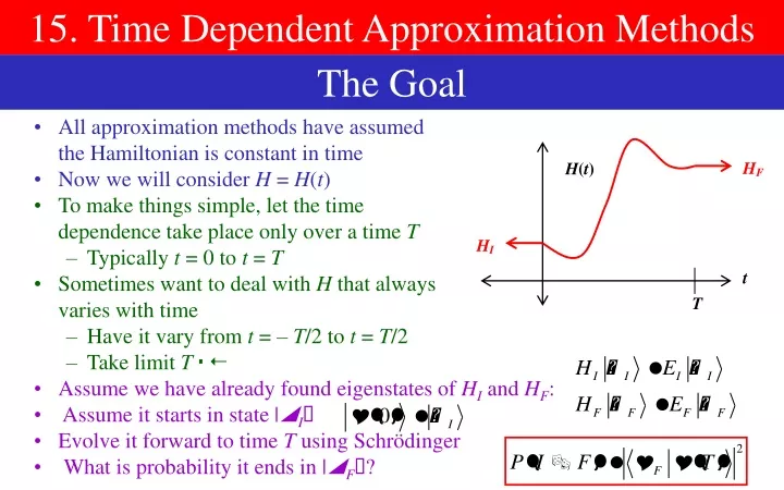
15. Time Dependent Approximation Methods. The Goal. All approximation methods have assumed the Hamiltonian is constant in time Now we will consider H = H ( t ) To make things simple, let the time dependence take place only over a time T Typically t = 0 to t = T

E N D
15. Time Dependent Approximation Methods The Goal • All approximation methods have assumedthe Hamiltonian is constant in time • Now we will consider H = H(t) • To make things simple, let the timedependence take place only over a time T • Typically t = 0 to t = T • Sometimes want to deal with H that alwaysvaries with time • Have it vary from t = – T/2 to t = T/2 • Take limit T • Assume we have already found eigenstates of HIand HF: • Assume it starts in state |I • Evolve it forward to time T using Schrödinger • What is probability it ends in |F?
15A. The Sudden Approximation Short Time = No Change • Suppose H changes quickly from HI to HF, T small • We must solve Schrödinger: • Since T is small, use Taylor expansion:
Comments On the Sudden Approximation • In general, though Fand Iare both eigenstates, they are eigenstates of different Hamiltonians When is this approximation valid? • The leading term we dropped was O(TH/) • H is of order the energies, so this is small if • Can show, only differences in energies matter, so really need • Probabilities are always pure numbers • If there are any dimensionful combinations in your answer, your answer is wrong • Answers should have a numerical answer 1
Sample Problem A particle is initially in the ground state of a Harmonic oscillator potential with frequency(t), where(t) changes from 0 to 20 very quickly (T 0 << 1). What is the probability it remains in the ground state? • The probability is: • The initial state has wave function • The final state has same wave function,with 0 changed to 20: • The overlap is
15B. The Adiabatic Approximation Instantaneous Eigenstates • Suppose H changes slowly from HI to HF, T large • Ateach moment, find eigenstates of Hamiltonian • Eigenstates are always orthonormal, therefore • Take time derivative: • Imaginary part is undetermined: • The eigenvalue equation for |i(t) is ambiguous up to a phase • By multiplying |i(t) by a time-dependent phase, we can make it whatever we want • We can choose imaginary part to vanish too, so
State Vector in Terms of Eigenstates • Let’s write |(t) in terms of our eigenstates • Substitute intoSchrödinger’s Equation: • Take inner product with one state n(t)|:
Pulling Out the Large Phase • Because Hamiltonian is changing slowly, eigenstates are also changing slowly • Expect second term to be small • Solution to just first term is pretty easy • Let us define bnby • Substitute into differential equation:
Integrating the Equation • The term with i = n is absent because • Integrate to get the total change in bn(t): Derivatives are small because H is slowly changing • But integration is over long time! • But it’s multiplied by a phase that is constantly changing • So it should be small, just need to prove it • For each value of i and n,define the phase angle by • Note that • We therefore have:
The Approximation • Integrateby parts: • If we assume that (T) is large, then derivatives are small • Every term inside {} should be small, so • Recall that
Now We Tie It All Together • Recall what cn is: • Initial state assumed: • We want probability • It stays in the same state, of a different Hamiltonian • Normally, ground state ground state, first excited first excited, etc. • We explicitly assumed (T) is large • If we let E be typical energy splitting, then we are assuming • This is exact reverse criterion of sudden approximation
Sample Problem A particle is initially in the ground state of a Harmonic oscillator potential with frequency(t), where(t) changes from 0 to 20 very slowly (T 0 << 1). What is the probability it remains in the ground state? • The probability is:
Level Crossings • Sometimes, as the Hamiltonian evolves, eigenstates will have energies that approach each other • Adiabatic approximation applies only if we always have • Normally, the difference E will not vanish, because there will be mixing that causes the states to mix heavily as Hamiltonian changes • If there is mixing between the states, then we follow the general rule • Ground state ground state, etc. • Suppose we have a symmetry operator T thatcommutes with the Hamiltonian at all times • Then eigenstates will be eigenstates of both T and H: • As time evolves, eigenvalue under T will stay the same • The lowest energy state with the initial eigenvaluewill become the lowest energy state with the same eigenvalue, etc. • You can have level crossings betweenstates with different values of .
Sample Problem An electron in spin state |+ at t = – is in a region with time-dependent magnetic field . What state will it be in at t = + if: (a) eBx2 >> mb (b) Bx = 0 Bx = 0 Bx0 • The relevant Hamiltonian is: • Eigenvalue graph as a function of time: • Two spin states are mixed around t = 0 if Bx 0 • For characteristic time T ~ Bx/b • For part (a), the low energy state will remain the low energy states in adiabatic approximation: • Valid if • For part (b), the Hamiltonian always commutes with Sz • Therefore, Szeigenvalue will never change |– |+ |– |+
15C. Time-Dependent Perturbation Theory Setting Up the Problem • Consider a Hamiltonian with a small time-dependent part • Assume we know the eigenstates and eigenvalues of H0 • W(t) is assumed to be small • These states are a complete, orthonormal basis • We can write the state vector in terms of these states • Assume we start in state |I and want probability we end in state |F
Schrödinger’s Equation • We now write out Schrödinger’s equation • Take inner product with n|
Pulling Out the Large Phase • If W is small, we expect second term to be small • In absence of second term, solution to first is cn ~ exp(–iEnt/) • We therefore define: • Substitute in: • Define the frequency differenceand matrix element: • We therefore have:
Integrating and Working on Answer • Integrate to time T: • Recall: • Therefore • Recall: • Define: • Then we have:
Making a Series Expansion • Substitute this expression into itself repeatedly • We have a perturbative expansion for the transition
Comments on Perturbative Expansion • We almost never interested in cases where F = I • Ignore first term • If we include only thesecondterm, then we get • Not hard to show that SFI is a unitary matrix • Closely related to U(T,0) being a unitary operator
Sample Problem A hydrogen atom is in state |1,0,0 when it is subjected to a temporary electric field given by . What is the probability it transitions to state |n,l,m ? • Electric field comes from scalar potential and/orvector potential • We can use: • This adds perturbation • Matrixelement is • Normally, run time integral from 0 to T, but in this case, from – to + • We have: • Non-zero only for l = 1, m = 0 • Vanishes if T = 0 (sudden approximation) • Vanishes if T = (adiabatic approx.)
15D. Harmonic Perturbations Harmonic Perturbations • It is very common to have the perturbation looklike a sine or a cosine • These can be rewritten: • Define a harmonic perturbation as one of the form: • Assume 0 • We will use our perturbation expansion,but assume F I, and only keep first order • We actually want to think of the perturbation as always present • Make t run from – T/2to +T/2; later take limit T • Define WFIas • Then we have • Substitute in:
Large Effects Near Resonance • Do the integrals: • In general, if W is small, expect these terms to be small • Unless we have a small denominator! • We will approximate two cases: • Where FI (energy increasing) • Where FI – (energy decreasing) • In each of these cases, we will only keeptrack of the large term, and ignore the other
Energy Increasing Case – Large T limit • We want transition probability: • Consider limit T • Look at function in {}’s: • As T , it looks like a delta function • To find the coefficient A,integrate both sides over all • Let Maple do the work,or use contour integration
Some Reminders on Delta-Functions • General integralof a delta function: • This allows you torewrite delta functions • In particular, • We therefore have • Recall that: • So
Transition Rates • Note that probability is proportional to T • The longer you wait, the more likely you are to have a transition • Define the rate as the probability per unit time • This formula assumed EF > EI, we still need to do the other case • Then put the formulas together: • Note energy is not conserved • Not surprising for a non-constant Hamiltonian • Note the energy change is • This energy is being added/subtracted from a classical background source • Later we’ll realize this is photon energy
Reverse Transitions • Consider a case where EF > EI, and we consider F I • Rate for forwards and backwards transitionsare the same! • Implies that in a thermal background, excited/ground states will eventually become equally populated • We’ll correct this false impression when we quantize EM fields
What to Do With the Delta Functions • How should we handle the delta functions? • Naively, we would always get zero or infinity • The frequency might be changing with time • There might be many frequencies present • We’ll use this in a later chapter • There may be multiple final states that need to be added up, which can be converted to an integral • For example, final states are free particles • Deal with this in next section • If experiment is finite time, you can simply not take the limit T • It ends up not quite a delta function
Sample Problem A harmonic oscillator with mass m and angular frequency 0 is in the ground state |0 at t = 0, and is subjected to a perturbation . The angular frequency of the driving perturbation is gradually adjusted to increase, so = t. To first order in perturbation theory, what state can it transition to, and what is the corresponding probability? • Since in the ground state,it can only go up in energy • Need to write perturbation in the form • We need the matrix element:
Sample Problem (2) A harmonic oscillator with mass m and angular frequency 0 is in the ground state |0 at t = 0, and is subjected to a perturbation . The angular frequency of the driving perturbation is gradually adjusted to increase, so = t. To first order in perturbation theory, what state can it transition to, and what is the corresponding probability? • This is the rate at any given time • We integrate this rate to get the total probability
Sample Problem A hydrogen atom in its ground state is in a region of rapidly oscillating electric field in the z-direction, Ez= E0cos(t), where is much larger than the binding energy of hydrogen. What is the rate at which it will dissociate the electron? • As usual, we have • Initial state is ground state of hydrogen: • EF will be large, so large that the finalelectron will effectively be a free electron • The electric potential is easily found • This lets us get the perturbation: • We now need the matrix element
Sample Problem (2) A hydrogen atom in its ground state is in a region of rapidly oscillating electric field in the z-direction, Ez= E0cos(t), where is much larger than the binding energy of hydrogen. What is the rate at which it will dissociate the electron?
Sample Problem (3) A hydrogen atom in its ground state is in a region of rapidly oscillating electric field in the z-direction, Ez= E0cos(t), where is much larger than the binding energy of hydrogen. What is the rate at which it will dissociate the electron? • After a lotof work: • The energy of the final states is • Decay rate to a particular k is: • The states |k are continuum states • We can go into any |k to dissociate
15E. EM Waves and the Dipole Approximation The Perturbation • Consider the effects of an external electromagnetic field on an atom • We start with the Hamiltonian: • The potential Vacontains all the internal interactions of the atom with itself • The unperturbed Hamiltonian is just: • Assume we know the eigenstates |a • Assume the external fields are small • Only keep first order in A • The perturbation will be: • We implicitly assumed PA = AP • Works if A = 0 • We’ll justify this assumption shortly
The Waves • We now need to make an electromagnetic wave • Multiple ways to do this, but oneway (Coulomb gauge) is to use: • The polarization vector is a normal vector perpendicular to k: • Note that this satisfies A = 0 • Moves at speed c: • The electric andmagneticfields are: • So we have: • Compare with: • So we have:
The Dipole Approximation • We will need matrix elements • Atomic states have size ~ a0 • We will typically be working with waves with energy of order the binding energy of the atom • We therefore will have • Therefore, kRj << 1 • The relative size of the secondterm compared to the first is: • We make the electric dipole approximation:
Working With the Dipole Approximation • There is a better way to work out this matrix element. Consider: • It follows that: • Our rate is therefore:
Rewrite in Terms of Intensity • You can’t measure the vector potential A, just the fields E and B • Most commonly, you measure the intensity , the power per unit area • Computed in E&M as the time-averaged magnitude of the Poynting Vector: • Time average and expand out the triple cross products: • Use that is normalized and orthogonal to k • The intensity is therefore • And we therefore have
Putting it All Together • Define the dipole matrix element • Speed of light,from E&M: • Recall • Substitute in: • Fine structure constant: • Delta function assures that = FI, so this simplifies to:
Dealing With the Dirac Delta Function • How do we deal with the delta function? • Often, incident light has a range of frequencies: • Logically, should be called d/d, but it isn’t • Other measures ofintensity are related: • Replace byan integral: • So we have:
Averaging Over Polarization, And Direction • Formula assumes we know the polarization • If incident light is unpolarized, need to averagethe two polarizations perpendicular to k • For example, let’s assume rFI is real • Let be angle between k and rFI • One polarization can be chosen in the plane of k and rFI • The other is perpendicular to both k and rFI • The rate, averaged overpolarizations will be: • If direction of light (or orientationof atom) is random, we can alsoaverage over angles
Comments on Electric Dipole Rate • If you know the polarization, you don’t need all components of rFI • Just calculate the component you need: Only certain states have non-zero matrix elements • Non-zero only if • Because operator R is parity -1, initial and final states must have opposite parity • This is automatically assured by l = 1 for Hydrogen, but not for other atoms • If l 1, then electric dipole can’t cause transition • But higher order interactions can
Sample Problem An electron is trapped in the ground state of a cubical box of size a3, with a corner at the origin. It is then bathed in light moving in the z-direction,polarized in the x-direction, and having intensity function (). In the dipole approximation, (a) which states can the electron transition into, (b) what are the corresponding frequencies , and (c) what are the transition rates • We first need the eigenstatesand eigenergies of the electronin the box: • Polarization is • We need matrix element • Only states possible are|n11 with n even
Sample Problem (2) (b) what are the corresponding frequencies , and (c) what are the transition rates • The frequencies are (n is even): • The rate is:
15F. Beyond the Dipole Approximation Higher Order Terms • Recall: • We dropped second term and kRj because they were smaller by factors of ka0 ~ • So, keep them toone more order • First term leads toelectric dipole term • For the second term,use this identity: • Rewrite as • Newterms:
Electric Quadrupole and Magnetic Dipole • Last term: • Magnetic dipole term: • We’ll set this aside and let you work on it with homework • The remaining term is the electric quadrupole term:
Simplifying the Electric Quadrupole Term • As before, we can use a clever commutator to simplify: • So we have:
Simplifying the Electric Quadrupole Term (2) • Let H0 act to theleft or to the right,as before • Now get the rate: • As usual, convert to intensity
Putting It Together • Use fine structure constant • As before, = FI because of the delta function • Integrate over • Final answer:
Comments on E2 and M1 transition • Electric quadrupole term2 tends to be down by factor of (ka0)2 ~ 2 compared to electric dipole • Same can be proven about the magnetic dipole contribution The electric quadrupole term can be shown to be a rank-2 spherical tensor • Means that |l| = 0, 1 or 2 Both electric quadrupole and magnetic dipole commute with parity • Connect only same parity states • Unlike electric dipole, which reverses parity • Means no interference with electric dipole Magnetic dipole operator commutes with H0 • Only connects states that are split by smaller effects • Spin orbit • Hyperfine • External B-field
Sample Problem An electron is trapped in the ground state of a cubical box of size a3, with a corner at the origin. It is then bathed in light moving in the z-direction,polarized in the x-direction, and having intensity function (). In the electric quadrupole approximation, (a) which states can the electron transition into, (b) what are the corresponding frequencies , and (c) what are the transition rates • We first need the eigenstatesand eigenergies of the electronin the box: • Polarization is • We need matrix element • Only states possible are|n1p with n,p even