Download
1 / 32
320 likes | 437 Views
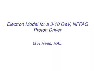
3 GeV, 1.2 MW, RCS Booster and 10 GeV, 4.0 MW, NFFAG Proton Driver. G H Rees, ASTeC, RAL. Introduction. Studies for the ISS: 1. Proton booster and driver rings for 50 Hz, 4 MW and 10 GeV. 2. Pairs of triangle and bow-tie, 20 (50 GeV) ± decay rings. Studies after the ISS:

E N D
3 GeV, 1.2 MW, RCS Booster and 10 GeV, 4.0 MW, NFFAG Proton Driver G H Rees, ASTeC, RAL
Introduction Studies for the ISS: 1. Proton booster and driver rings for 50 Hz, 4 MW and 10 GeV. 2. Pairs of triangle and bow-tie, 20 (50 GeV) ± decay rings. Studies after the ISS: 1. A 3 - 5.45 MeV electron model for the 10 GeV, proton NFFAG. 2. An alternative proton driver using a 50 Hz, 10 GeV, RCS ring. 3. A three pass, ± cooling, dog-bone re-circulator
Proton Driver Parameter Changes for ISS • Pulse repetition frequency F = 15 to 50 Hz • 4 MW, proton driver energy T = (8 or 26) to 10 GeV • No. of p bunches & μ± trains n = 1 to (3 or 5) Reasons for the changes: • For adiabatic proton bunch compression to ~ 2 ns rms • For lower peak & average beam currents in μ± rings • To allow partial beam loading compensation for the μ±
Bunch Train Patterns 1 1 (h=3, n=3) (h=24, n=3) (h=5, n=5) (h=40, n=5) NFFAG 2Rb , Tp Tp= Td /2 RCS ( Rb ) . 3 2 2 3 μ±bunch rotation P target Acceler. of trains of 80 μ± bunches 1 NFFAG ejection delays: (p + m/n) Td for m = 1 to n (=3,5) Pulse < 40 μs for liquid target Pulse > 60 μs for solid target Decay rings, Td h = 23335 3 2 80 μˉ orμ+bunches
Schematic Layout of 3 GeV, RCS Booster 200 MeV H ˉ H ˉ, H° beam cavities collectors dipoles 8° dipole dipoles R = 63.788 m n = h = 3 or 5 triplet triplet extraction cavities
Parameters for 50 Hz, 0.2 to 3 GeV Booster • Number of superperiods 4 • Number of cells/superperiod 4(straights) + 3(bends) • Lengths of the cells 4(14.0995) + 3(14.6) m • Free length of long straights 16 x 10.6 m • Mean ring radius 63.788 m • Betatron tunes (Qv, Qh) 6.38, 6.30 • Transition gamma 6.57 • Main dipole fields 0.185 to 1.0996 T • Secondary dipole fields 0.0551 to 0.327 T • Triplet length/quad gradient 3.5 m/1.0 to 5.9 T m-1
Beam Loss Collection System . Main dipoles Primary H,V Secondary Collectors Local shielding Collimators μ = 90° μ =160° Momentum collimators Radiation hard magnet Triplet Secondary p collector
Choice of Lattice • ESS-type, 3-bend achromat, triplet lattice chosen • Lattice is designed around the Hˉ injection system • Dispersion at foil to simplify the injection painting • Avoids need of injection septum unit and chicane • Separated injection; all units between two triplets • Four superperiods, with >100 m for RF systems • Locations for momentum and betatron collimation • Common gradient for all the triplet quadrupoles • Five quad lengths but same lamination stamping • Bending with 20.5° main & 8° secondary dipoles
Schematic Plan of Hˉ Injection . Optimum field for n = 4 & 5, H°Stark state lifetimes. 0.0551 T, Injection Dipole Hˉ H+ Stripping Foil Septum input Hˉ H° H+ Foil 8° 5.4446 m • V1 V2 Vertical steering/painting magnets V3 V4 • Horizontal painting via field changes, momentum ramping & rf steering • Separated system with all injection components between two triplets. • Hˉ injection spot at foil is centred on an off-momentum closed orbit.
Electron Collection after Hˉ Stripping Cooled copper graphite block Foil support 109 keV, 90 W, eˉ beam Stripping Foilρ = 21.2 mm, B = 0.055 T . H° H° 200 MeV, 80 kW, Hˉ beam 5 mm 170 injected turns, 28.5 (20 av.) mA Protons Protons Foil lattice parameters : βv = 7.0 m, βh = 7.8 m, Dh = 5.3 m, Dh /√ βh = 1.93 m½ Hˉ parameters at stripping foil ; βv = 2.0 m, βh = 2.0 m, Dh = 0.0 m, Dh' = 0.0
Anti-correlated, Hˉ Injection Painting Y Vertical acceptance Hˉ injected beam Initial closed orbits Final closed orbits Collapsed closed orbits Δp/p spread in X closed orbits Small v, big h amplitudes at start Small h, big v amplitudes at end. Foil . ------------------------------------ oHˉ o ½painted ε(v) --------------------------------------------- --------------------------- ------------- OX ½painted ε(h) Collimator acceptance Horizontal acceptance For correlated transverse painting : interchange X closed orbits
Why Anti-correlated Painting? Assume an elliptical beam distribution of cross-section (a, b). The transverse space charge tune depressions/spreads are : δQv = 1.5 [1 - S/ ∫(βv ds / b(a+b))] δQv (uniform) 4S = ∫[βv /b(a+b)2] [(y2 (a + 2b)/ 2b2 ) + (x2/a)] ds Protons with (x = 0, y = 0) have δQv = 1.5 δQv (uniform distrib.) Protons with (x = 0, y = b) have δQv ~ 1.3 δQv (uniform distrib.) Protons with (x = a, y = 0) or (x = a/2, y= b/2) have ~ 1.3 factor. δQ shift is thus less for anti-correlated than correlated painting. The distribution may change under the effect of space charge.
Emittances and Space Charge Tune Shifts Design for a Laslett tune shift (uniform distribution) of δQv = 0.2. An anti-correlated, elliptical, beam distribution has a δQv = 0.26. For 5 1013 protons at 200 MeV, with a bunching factor of 0.47, the estimated, normalised, rms beam emittances required are: εσ n = 24 (π) mm mrad εmax = 175 (π) mm mrad The maximum, vertical beam amplitudes (D quads) are 66 mm. Maximum, horizontal beam amplitudes (in F quads) are 52 mm. Maximum, X motions at high dispersion regions are < 80 mm. Max. ring/collimator acceptances are 400/200 (π) mm mrad.
Fast Extraction at 3 GeV K1 K2 K3 K4 F D F 10.6 m straight section F D F . • Fast kicker magnets Triplet Septum unit Triplet • Horizontal deflections for thekicker and septum magnets • Rise / fall times for 5 (3) pulse, kicker magnets = 260 ns • Required are 4 push-pull kickers with 8 pulser systems • Low transverse impedance for (10 Ω) delay line kickers • Extraction delays, ΔT, from the booster and NFFAG rings • R & D necessary for the RCS and the Driver pulsers
RF Parameters for 3 GeV Booster • Number of protons per cycle 5 1013 (1.2 MW) • RF cavity straight sections 106 m • Frequency range for h = n = 5 2.117 to 3.632 MHz • Bunch area for h = n = 5 0.66 eV sec • Voltage at 3 GeV for ηsc < 0.4 417 kV • Voltage at 5 ms for φs = 48° 900 kV • Frequency range for h = n = 3 1.270 to 2.179 MHz • Bunch area for h = n = 3 1.1 eV sec • Voltage at 3 GeV for ηsc < 0.4 247 kV • Voltage at 5 ms for φs = 52° 848 kV
Schematic Layout of Booster and Driver 3 GeV RCS booster 66 cells 10 GeV NFFAG H°, Hˉ Hˉ collimators 200 MeV Hˉ linac
Homing Routines in Non-linear, NFFAG Program • A linear lattice code is modified for estimates to be made of the non-linear fields in a group of FFAG magnets. • Bending radii are found from average field gradients between adjacent orbits & derived dispersion values, D. • D is a weighted, averaged, normalized dispersion of a new orbit relative to an old, and the latter to the former. • A first, homing routine obtains specified betatron tunes. A second routine is for exact closure of reference orbits • A final, limited-range, orbit-closure routine homes for -t. Accurate estimates are made for reference orbit lengths. • Full analysis needs processing the lattice output data & ray tracing in 6-D simulation programs such as Zgoubi.
Non-linear Fields and Reference Orbits • Low ampl. Twiss parameters are set for a max. energy cell. • Successive, adjacent, lower energy reference orbits are then found, assuming linear, local changes of the field gradients. • Estimates are repeated, varying the field gradients for the required tunes, until self-consistent values are obtained for: the bending angle for each magnet of the cell the magnet bending radii throughout the cell the beam entry & exit angle for each magnet the orbit lengths for all the cell elements, and the local values of the magnet field gradients
The Non-linear, Non-scaling NFFAG • Cells have the arrangement: O-bd-BF-BD-BF-bd-O • The bending directions are : - + + + - • Number of magnet types is: 3 • Number of cells in lattice is: 66 • The length of each cell is: 12.14 m • The tunes, Qh and Qv ,are: 20.308 and 15.231 • Non-isochronous FFAG: ξv≈ 0 and ξh≈ 0 • Gamma-t is imaginary at 3 GeV, and ≈ 21 at 10 GeV • Full analysis needs processing non-linear lattice data & ray tracing in 6-D simulation programs such as Zgoubi
Lattice Cell for the NFFAG Ring bd(-) BF(+) BD(+) BF(+) bd(-) 2.2 0.62 1.29 1.92 (m) 1.29 0.62 2.2 –1.65° 3.5523° 1.65° 3.5523° –1.65° Lengths and angles for the 10.0 GeV closed orbit
Gamma-t vs. for the Driver and E-model Proton Driver Electron Model =E/Eo gamma-t =E/Eo gamma-t • 11.658 21.8563 11.658 19.9545 • 10.805 23.1154 10.980 22.4864 • 10.379 23.9225 10.393 24.2936 • 9.953 24.8996 9.806 28.9955 • 9.100 27.6544 9.219 51.1918 • 8.673 29.7066 8.632 34.7566 i • 8.247 32.5945 8.045 19.6996 i • 7.608 40.0939 7.458 14.2350 i • 6.968 64.0158 6.871 11.8527 i • 4.197 18.9302 i (imag.) – –
Loss Levels for NFFAG Proton Driver • Beam power for the 50 Hz Proton Driver = 4 MW • Total loss through the extraction region < 1 part in104 • Average loss outside coll./ extr. region < 1 part in104 • Total loss in primary & sec. collimators = 1 part in103 • Remotely operated positions for primary collimators. • Quick release water fittings and component flanges. • Local shielding for collimators to reduce air activation.
Vertical Collimation in the NFFAG Loss collectors Y . X 3 GeV proton beam 10 GeV proton beam Coupling may limit horizontal beam growth
Loss Collection for the NFFAG • Vertical loss collection is easier than in an RCS • ΔP loss collection requires beam in gap kickers • Horizontal beam collimation prior to the injection • Horizontal loss collection only before the ejection • Minimize the halo growth during the acceleration • Minimise non-linear excitations as shown later.
NFFAG Loss Collection Region 20° 160° Primary collimators (upstream end of 4.4 m straight) • Direct beam loss localised in the collection region • Beam 2.5 σ, Collimator 2.7 σ and Acceptance 4 σ p beam Cell 1 Cell 2 Cell 3 Secondary collectors
NFFAG Non-linear Excitations Cells Qh Qv 3rd Order Higher Order 4 0.25 0.25 zero nQh=nQv & 4th order 5 0.20 0.20 zero nQh=nQv & 5th order 6 0.166 0.166 zero nQh=nQv & 6th order 9 0.222 0.222 zero nQh=nQv & 9th order 13 4/13 3/13 zero to 13th except 3Qh=4Qv Use (13 x 5 ) + 1 = 66 such cells for the NFFAG Variation of the betatron tunes with amplitude? -t imaginary at low energy and ~ 20 at 10 GeV
Bunch Compression at 10 GeV For 5 proton bunches: Longitudinal areas of bunches = 0.66 eV sec Frequency range for a h of 40 = 14.53-14.91 MHz Bunch extent for 1.18 MV/ turn = 2.1 ns rms Adding of h = 200, 3.77 MV/turn = 1.1 ns rms For 3 proton bunches: Longitudinal areas of bunches = 1.10 eV sec Frequency range for a h of 24 = 8.718-8.944 MHz Bunch extent for 0.89 MV/ turn = 3.3 ns rms Adding of h = 120, 2.26 MV/turn = 1.9 ns rms Booster and Driver tracking studies are needed
50 Hz,10 GeV, RCS Alternative • Same circumference as for the outer orbit of the NFFAG • Same box-car stacking scheme for the ±decay rings • Same number of proton bunches per cycle (3 or 5) • Same rf voltage for bunch compression (same gamma-t) • Increased rf voltage for the proton acceleration (50% ?) • 3 superperiods of (15 arc cells and 6 straight sections) • 5 groups of 3 cells in the arcs for good sextupole placings • 2 quadrupole types of different lengths but same gradient • 2 dipole magnet types, both with a peak field of 1.0574 T
10 GeV NFFAG versus RCS Pros: • Allows acceleration over more of the 50 Hz cycle • No need for a biased ac magnet power supply • No need for an ac design for the ring magnets • No need for a ceramic chamber with rf shields • Gives more flexibility for the holding of bunches Cons: • Requires a larger (~ 0.33 m) radial aperture • Needs an electron model to confirm viability
R & D Requirements Development of an FFAG space charge tracking code. Tracking with space charge of booster and driver rings. Building an electron model for NFFAG proton driver. Magnet design & costing for RCS, NFFAG & e-model. . Development of multiple pulse, fast kicker systems. Site lay-out drawings & conventional facilities design NFFAG study (with beam loading) for μ±acceleration