Download
1 / 12
120 likes | 243 Views
Theory and Application of Multiple Regression Model. SUMBER: www.aaec.ttu.edu/faculty/omurova/aaec_4302/Lectures/Chapter_7. ppt . Pendahuluan. The multiple regression model aims to and must include all of the independent variables X1, X2, X3, …, Xk that are believed to affect Y

E N D
Theory and Application of Multiple Regression Model SUMBER: www.aaec.ttu.edu/faculty/omurova/aaec_4302/Lectures/Chapter_7.ppt
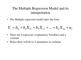
Pendahuluan • The multiple regression model aims to and must include all of the independent variables X1, X2, X3, …, Xk that are believed to affect Y • The multiple linear regression model is given by: Yi = β0 + β1X1i + β2X2i + β3X3i +…+ βkXki + ui where i=1,…,n represents the observations, k is the total number of independent variables in the model, β0, β1,…, βk are the parameters to be estimated, and ui is the disturbance term SUMBER: www.aaec.ttu.edu/faculty/omurova/aaec_4302/Lectures/Chapter_7.ppt
Example SUMBER: www.aaec.ttu.edu/faculty/omurova/aaec_4302/Lectures/Chapter_7.ppt
Y X2 Regression surface (plane) E[Y] = βo+β1X1+β2X2 Ui X2 slope Measured by β2 βo X1 slope measured by β1 X1 SUMBER: www.aaec.ttu.edu/faculty/omurova/aaec_4302/Lectures/Chapter_7.ppt
Pendugaan Model SUMBER: www.aaec.ttu.edu/faculty/omurova/aaec_4302/Lectures/Chapter_7.ppt
Interpretasi Koefisien ^ • The intercept βo estimates the value of Y when all of the independent variables in the model take a value of zero • In our example βo , is 144.94, which means that if : • Yi = 144.94+β1*(0)+β2*(0) + β3*(0)+β4*(0) • All the independent variables take the value of zero (price of beef is zero cents/lb, price of chicken is zero cents/lb, price of pork is zero cents/lb, and the income for US population is zero dollars/ per – year, then the estimated beef consumption will be 144.94 lbs/year). ^ ^ ^ ^ ^ SUMBER: www.aaec.ttu.edu/faculty/omurova/aaec_4302/Lectures/Chapter_7.ppt
Interpretasi Koefisien ^ ^ ^ • In a strictly linear model, β1, β2,..., βk are slopes of coefficients that measure the unit change in Y when the corresponding X (X1, X2,..., Xk) changes by one unit and the values of all of the other independent variables remain constant at any given level • Ceteris paribus (other things being equal) SUMBER: www.aaec.ttu.edu/faculty/omurova/aaec_4302/Lectures/Chapter_7.ppt
InterpretasiKoefisien ^ • In our example: • β1= -0.00291. That means, if the price of beef increases by one cent/lb then the beef consumption will decrease by 0.00291 pounds per – year, ceteris paribus • β2= -0.116. That means, if the price of chicken increases by one cent/lb then the beef consumption will decrease by 0.116 pounds per – year, ceteris paribus (Does this result makes sense?) ^ SUMBER: www.aaec.ttu.edu/faculty/omurova/aaec_4302/Lectures/Chapter_7.ppt
Kecocokan (Kesesuaian) Model i=1 i=1 • R2 = 1 - { ei2/ (Yi-Y)2} • A disadvantage of R2 is that it always increases in value as independent variables are added into the model SUMBER: www.aaec.ttu.edu/faculty/omurova/aaec_4302/Lectures/Chapter_7.ppt
Kecocokan (Kesesuaian) Model • The adjusted or corrected R2 : • R2 = 1 [{ei2/(n-k-1)}/{(Yi-Y)2/(n-1)}] • The R2 is always less than the R2, unless the R2 = 1 • Adjusted R2 lacks the same straightforward interpretation as the regular R2 SUMBER: www.aaec.ttu.edu/faculty/omurova/aaec_4302/Lectures/Chapter_7.ppt
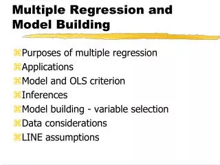
The Specification Question • Any variable that is suspected to directly affect Y should be included in the model • Excluding such a variable would likely cause the estimates of the remaining parameters to be “incorrect”; i.e. biased SUMBER: www.aaec.ttu.edu/faculty/omurova/aaec_4302/Lectures/Chapter_7.ppt
FungsiPendapatan • Multiple regression model of the earnings: EARNGSi = β0 + β1EDi + β2EXPi + ui • Cross-section data set, 100 observations EARNGSi =-6.179+0.978EDi+0.124EXPi R2 = 0.315 Adj.R2 = 0.298 SUMBER: www.aaec.ttu.edu/faculty/omurova/aaec_4302/Lectures/Chapter_7.ppt