Download
1 / 40
420 likes | 618 Views
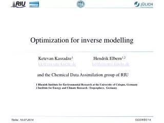
Optimization for inverse modelling. Ketevan Kasradze 1 Hendrik Elbern 1,2 kk@riu.uni-koeln.de he@riu.uni-koeln.de and the Chemical Data Assimilation group of RIU 1 Rhenish Institute for Environmental Research at the University of Cologne, Germany

E N D
Optimization for inverse modelling Ketevan Kasradze1 Hendrik Elbern1,2 kk@riu.uni-koeln.dehe@riu.uni-koeln.de and the Chemical Data Assimilation group of RIU 1 Rhenish Institute for Environmental Research at the University of Cologne, Germany 2 Institute for Energy and Climate Research -Troposphere, Germany
Atmospheric layers 3/18
Atmospheric layers SACADA 3/18
SACADA assimilation-system Background Meteorological ECMWF analyses Trace gas observations PREP SACADA DWD GME CTM CTMad Diffusion L-BFGS Analysis
Horizontal GME Grid • ~147km between the grid points • 23 042 grid points per Model layer 9/18
SACADAVerticalGrid 54 layer MLS Additional refinement troposphere/lower stratosphere CRISTA-NF
HNO3 4.11.2005 ~137hPa 12 Uhr UTC MLS 15
SCOUT-O3campaignStratospheric-Climate Links with Emphasis on the UTLS - O3November-December 2005 AMMA-campaignAfricanMonsoonMultidisciplinaryAnalyses 29.07.2006 -17.08.2006 12/18
SACADA assimilation-system 4D-Var Model operator Background Projection operator Cost function Observation error covariance matrix Background error covariance matrix BECM ~ 1012 ~ 80 Terrabyte Vector of observations
SACADA assimilation-system 4D-Var Gradient Adjoint Model
Quasi-Newton method L-BFGS SACADA assimilation-system 4D-Var
Quasi-Newton method L-BFGS SACADA assimilation-system 4D-Var Background error covariance matrix BECM ~ 1012 ~ 80 Terrabyte
Background error covariance matrix formulation Radius of Influence ((de-)correlation length):Extending the information from an observation location • For atmospheric chemistry covariance modelling the diffusion approach is advocated: • localisation intrinsically performed • sharp gradients easily feasible • matrix square roots for preconditioning straightforward to calculate; no inversion needed Textbook: horizontal influence radius L around a measurement site, to be based on a priori statistical assessments Horizontal structure function, to be stored as a column of the forecast error covariance matrix diffusion operator construction vertical cut L L
Isopleths of the cost function and transformed cost function and minimisation steps concentration species 2 transformed species 2 concentration species 1 transformed species 1 Minimisation by mere gradients,quasi-Newon method L-BFGS (Large dimensional Broyden Fletcher Goldfarb Shanno), and preconditioned (transformed) L-BFGS application
Background error covariance matrix formulation • 2 outstanding problems: • With linear estimation: How to treat the background error covariance matrix B (O(1012))? • How can this be treated for preconditioning? (need B-1, B1/2, B-1/2) With variational methods: Solution: Diffusion Approach Transformation of cost-function: minimisation procedure => Inverse of B and B-1/2 are not needed, if xb= 1. guess.
Background error covariance matrix formulation Background Observation: 3 ppm Ozone
Background error covariance matrix formulation Background Observation: 3 ppm Ozone Analysis (B diagonal)
Background error covariance matrix formulation Background Observation: 3 ppm Ozone
Background error covariance matrix formulation Background Observation: 3 ppm Ozone Analysis increment isotropic correlation The increment in initial values is spread out to neighbouring grid-points depending on the correlations that are known / assumed.
Background error covariance matrix formulation Diffusion can be generalised to account for inhomogeneous and anisotropic correlations: Stratospheric case use PV field for anisotropic correlation modelling Assumption: Strong correlation along isolines of Potential Vorticity Enhancement of diffusion flow-dependent BECM
Background error covariance matrix formulation Background Observation: 3 ppm Ozone
Background error covariance matrix formulation Background Observation: 3 ppm Ozone Analysis increment
Quasi-Newton method L-BFGS SACADA assimilation-system 4D-Var Adjoint Model
backward model (backward differential equation) forward model (forward differential equation) adjoint algorithm (adjoint solver) algorithm (solver) code adjoint code Construction of the adjoint code(3 different possible pathways)
Adjoint model A numerical model integration over a time interval [t0; ti] Accordingly, the tangent linear of this sequence of model operators is given by Thus, the adjoint model operator Mi propagates the gradient of the cost function with respect to xi backwards in time, to deliver the gradient of the cost function with respect to x0.
Quasi-Newton method L-BFGS SACADA assimilation-system 4D-Var Limited-memory Broyden–Fletcher–Goldfarb–Shanno algorithm
Gradient of the cost function h Hessian of the cost function
BFGS algorithm (2) From an initial guess x0 and an approximate Hessian matrix H0 the following steps are repeated as xk converges to the solution. Obtain a direction sk by solving: Perform a line search to find an acceptable step sizein the direction found in the first step, then update Set Convergence can be checked by observing the norm of the gradient, .
BFGS example with MATLAB it= 40 f=1.497581e-13 ||g||=1.726061e-05 sig=1.200 step=BFGS it= 41 f=5.990317e-15 ||g||=3.452127e-06 Successful termination with ||g||<1.000000e-08*max(1,||g0||):
Thank you for your attention!გმადლობთ ყურადღებისათვის!Vielen Dank für Ihre Aufmerksamkeit!