Download
1 / 36
360 likes | 525 Views
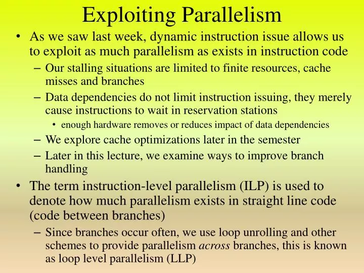
Exploiting Parallelism. As we saw last week, dynamic instruction issue allows us to exploit as much parallelism as exists in instruction code Our stalling situations are limited to finite resources, cache misses and branches

E N D
Exploiting Parallelism • As we saw last week, dynamic instruction issue allows us to exploit as much parallelism as exists in instruction code • Our stalling situations are limited to finite resources, cache misses and branches • Data dependencies do not limit instruction issuing, they merely cause instructions to wait in reservation stations • enough hardware removes or reduces impact of data dependencies • We explore cache optimizations later in the semester • Later in this lecture, we examine ways to improve branch handling • The term instruction-level parallelism (ILP) is used to denote how much parallelism exists in straight line code (code between branches) • Since branches occur often, we use loop unrolling and other schemes to provide parallelism across branches, this is known as loop level parallelism (LLP)
Multiple Issue • The next step to further exploit ILP is to issue multiple instructions per cycle • Send 2 or more instructions in 1 cycle to the execution units (reservation stations) • we call such a pipeline a superscalar pipeline • Two approaches • Static scheduling – instructions are grouped together by the compiler • Dynamic scheduling – using a Tomasulo-based architecture, instructions are issued in the order they are retrieved as found in the instruction queue, but if we can issue more than 1 at a time, we do • Simple example: • Issue 1 integer and 1 FP operation since they do not typically interact and so would not have dependencies • loads/stores are considered int even if the datum is FP • Superscalars can be set up to issue up to 8 instructions per clock cycle
Example Loop: L.D F0, 0(R1) L.D F1, 0(R2) ADD.D F2, F0, F1 L.D F3, 0(R3) L.D F4, 0(R4) ADD.D F5, F3, F4 SUB.D F6, F3, F2 DADDI R1, R1, #8 DADDI R2, R2, #8 DADDI R3, R3, #8 DADDI R4, R4, #8 DADDI R5, R5, #8 S.D F6, 0(R5) DSUBI R6, R6, #1 BNE R6, Loop Integer Loop: FP L.D F0, 0(R1) L.D F1, 0(R2) L.D F3, 0(R3) L.D F4, 0(R4) ADD.D F2, F0, F1 DADDI R1, R1, #8 DADDI R2, R2, #8 ADD.D F5, F3, F4 DADDI R3, R3, #8 DSUBI R6, R6, #1 DADDI R4, R4, #8 SUB.D F6, F3, F2 DADDI R5, R5, #8 BNE R6, Loop S.D F6, -8(R5) Stalls for the single issue code would be 1 after each of L.D F0, L.D F4, 3 after ADD.D, 1 after DSUBI and 1 in the branch delay slot, scheduling can remove a number of the stalls, using the 2 issue superscalar (without loop unrolling) provides the code to the right, which consists of 13 cycles of 15 instructions, a CPI = .87
Adding Loop Unrolling • Given the loop below, scheduling it for a superscalar would be futile • The only FP operation has a data dependence with the instructions that precede and succeed it • The best we could do is to schedule the DADDI and ADD.D together, moving the S.D down • to resolve this, we need to add loop unrolling to the process so that we have enough instructions to schedule • assume the ADD.D has a latency of 2 cycles between it and the S.D, we need to have 2 additional operations between it and the S.D Loop: L.DF2, 0(R1) ADD.DF2, F2, F0 S.DF2, 0(R1) DADDI R1, R1, #8 BNE R1, R2, Loop Solution: unroll the loop at least 3 iterations worth and schedule
Solution Integer FP Loop: L.D F2, 0(R1) L.D F4, 8(R1) L.D F6, 16(R1) ADD.D F2, F2, F0 L.D F8, 24(R1) ADD.D F4, F4, F0 DADDI R1, R1, #32 ADD.D F6, F6, F0 S.D F2, -32(R1) ADD.D F8, F8, F0 S.D F4, -16(R1) S.D F6, -8(R1) BNE R1, R2, Loop S.D F8, 0(R1) • CPI for this code is 14 instructions in 11 cycles • or 11/14 = .79 • with a superscalar that we can achieve a CPI < 1 • Note that if we unrolled the loop 3 times instead of 4, we would have 1 cycle where there was no int operation • Also note that the FP adder must be pipelined for this to work, from here on we will assume all FP functional units are pipelined
Another Solution • Assume we can issue any combination of instructions (that is, int or FP on either side of the superscalar) • Would this alter our solution? • We could still have the same solution, but we could also do this Instruction 1 Instruction 2 Loop: L.D F2, 0(R1) L.D F4, 8(R1) L.D F6, 16(R1) L.D F8, 24(R1) L.D F10, 32(R1) L.D F12, 40(R1) L.D F14, 48(R1) DADDI R1, R1, #56 ADD.D F2, F2, F0 ADD.D F4, F4, F0 ADD.D F6, F6, F0 ADD.D F8, F8, F0 ADD.D F10, F10, F0 ADD.D F12, F12, F0 ADD.D F14, F14, F0 S.D F2, -56(R1) S.D F4, -48(R1) S.D F6, -40(R1) S.D F8, -32(R1) S.D F10, -24(R1) BNE R1, R2, Loop S.D F12, -16(R1) S.D F14, -8(R1)
Dynamic Scheduling • With static issue, the compiler is tasked with finding instructions to schedule • With dynamic issue, the instructions must already be available to issue • Imagine our IF stage fetches 2 instructions per cycle, what are the chances that one is an int and one is a FP operation? • Can the hardware search through the instruction queue (the fetched instructions) to select two instructions? • there may not be enough time for that • Instead, we could issue 1 instruction per cycle, 2 if the instructions are int & FP • the following example demonstrates a typical loop being dynamically unrolled and issued 2 instructions at a time (without the 1 int + 1 FP restriction)
VLIW Approach • Related to the static superscalar approach is one known as the Very Long Instruction Word • Here, the compiler bundles instructions that can be issued together so that they can be fetched and issued as a bundle • Unlike the superscalar, the number of instructions scheduled together can be greatly increased • The combination of instructions scheduled together will reflect the available hardware units, for instance • Up to 2 load/stores • Up to 2 FP • Up to 2 integer • 1 branch • The instructions are bundled together so that the CPU fetches and issues 1 VLIW at a time • Loop unrolling is required to support this
Example: 5 Instruction VLIW Note that we do not fill the branch delay slot because we are using speculation. This code executes 7 iterations worth of the loop in only 9 cycles, providing a CPI of 9 / 23 = .39.
Supporting Superscalar • By expanding our architecture to a superscalar, we confront a serious problem • Recall from appendix A that branches make up perhaps 16% of a benchmark • Assuming a uniform distribution of instructions, this means that a branch occurs roughly every 6 instructions • for FP benchmarks, it may be more like every 8-9 instructions • There is just not enough instructions within a basic block (between branches) to obtain enough instructions to issue multiple instructions per cycle • Loop unrolling is one approach to handle this, but in general, to support multiple issue, we need instruction speculation • that is, we need to speculate which instruction(s) should next be fetched and/or scheduled
Branch Handling Schemes • For our pipeline, we used a branch delay slot or assumed branches were not taken • We could also use branch prediction to predict taken or not taken to control whether we immediately take the branch as soon as the new PC value is taken or not • this is only useful in longer pipelines where the branch location is computed earlier in the pipeline than the branch condition • the prediction is made using a cache, addressed by the instruction’s address (or some bits of the address) • Static branch prediction • Accumulate statistics on each branch in a program and base the branch prediction on those earlier runs • see figure C.17 (p C-27) which demonstrates miss-prediction rates on some SPEC92 benchmarks of between 5% and 22% • Static approach is not ideal because it does not consider the behavior of the current program
Dynamic Branch Prediction • For each branch, we store a single bit to indicate if that branch was last taken or not taken • If the buffer (cache) says “taken”, we will assume the branch should be taken and if the buffer says “not taken”, we will assume the branch should not be taken • If the prediction is incorrect, we modify the buffer • There is a problem with this simple approach • Assume we have a for loop which iterates 100 times • the first prediction is “not taken” • we have never been here before or the last time we were here, we exited the for loop and the branch was not taken • we reset our prediction bit to “taken” and predict correctly for the next 98 iterations • in the last iteration, we predict taken but the branch is not taken • 2 miss-predictions out of 100 (98%), can we improve?
Improved Scheme • An alternative approach is to use a 2-bit scheme • In general, it takes 2 miss-predictions to change our next prediction so we would miss-predict 1 time out of 100 • We can extend this to be an n-bit scheme which store the result of n previous branches, if the value >= 2n-1 / 2, we predict taken See table C.19 which shows the accuracy of the 2-bit predictor on several SPEC89 benchmarks – average miss-prediction is about 7% An n-bit predictor provides little improvement over the 2-bit scheme
Other Branch Prediction Schemes if(aa==2) aa=0; if(bb==2) bb=0; if(aa!=bb) … DSUBI R3, R1, #2 BNEZ R3, L1 DADD R1, R0, R0 L1: DSUBI R3, R2, #2 BNEZ R3, L2 DADD R2, R0, R0 L2: DSUB R3, R1, R2 BEQZ L3 • We want to improve over even the 2-bit scheme because of the amount of speculation required to support our superscalar • Consider the code above to the right • An analysis shows that if the first two branches are taken, then the third branch will not be taken • The equivalent MIPS code might look like that shown to the right
Correlating Branch Predictors • Although the previous example is probably not very common, it demonstrates that some branches can be predicted, at least in part, in correlation with other branches • A compiler may recognize the correlation • The problem with the branch prediction scheme (whether 1-bit, 2-bit or n-bit) is that it stores information only local to the one branch • Another approach is to have several predictors and choose the predictor based on the result of several recent branches • A correlating (or 2-level) predictor can provide more accurate predictions • The top level contains the locations of various predictors based on the result of more than one branch • Based on the top level, a different prediction is consulted • Both the top level and the branch predictor can be altered over time
Continued • An (m, n) predictor uses the behavior of the last m branches • to choose from 2m branch predictors • each branch predictor is an n-bit predictor • A (1, 2) predictor only uses the behavior of the last branch and selects a 2-bit predictor, this is what we had previously • A (2, 2) predictor might be useful for our previous example of if(aa!=bb) because it will select a 2-bit predictor • based on whether aa==2 or aa!=2 and whether bb==2 or bb!=2 • An (m, n) predictor scheme will require a buffer of 2m * n * k bits where k is the number of branches that we want to store predictions for • If we wanted to use a (2, 2) prediction scheme for 1K branches, it would take 22 * 2 * 1K = 8Kbits or 1KByte • remember, this is stored in an on-chip cache
Tournament Predictors • The tournament prediction scheme extends the correlating predictor by having multiple predictors per branch • At least one global and one local • The prediction is created as a combination of the various predictors • we won’t go over the details here • The chart to the right compares 2-bit predictor schemes, the top two being non-correlating predictors of 4096 and unlimited entries and the bottom being a (2, 2) correlating predictor using both local and global data
More Results Miss-prediction rates given total predictor size and type of predictors Overall miss-prediction rate FP predictions are more accurate than int predictions probably because there are more and lengthier loops in FP benchmarks
Branch Target Buffer • Our prediction schemes so far only store the prediction itself, not where the branch, if taken, is taking us • For some architectures, a pure prediction without a target location makes sense, recall the MIPS R4000 pipeline where the branch target was computed earlier in the pipeline than the branch prediction • However, for our superscalars, it would be necessary for us to know the predicted PC value as well as the prediction The branch target buffer, shown to the right, stores for each PC value, a predicted PC value To be most efficient, we would only want to cache branch instructions
Using the Branch Target Buffer • We fetch the branch prediction & target location in the IF stage from the buffer (an on-chip cache) at the same time we fetch the instruction • Is instruction a branch and branch is predicted as taken? • immediately change the PC to be the target location • if cache hit and successful prediction, penalty = 0 • Is instruction a branch and predicted to not be taken? • just increment PC as normal • if cache hit and successful prediction, penalty = 0 • Is instruction not a branch? • increment PC, no penalty • We have two sources of branch penalty • the branch is predicted as taken but is not taken (this is a buffer hit with a miss-prediction) • the branch is taken but is not currently in the buffer (a miss)
Performance of Branch Target Buffer • In MIPS, the penalty is a 2 cycle stall • One cycle to know the result of the branch as computed in the ID stage • One cycle to modify the cache (on a miss or miss-prediction) • many high performance processors have lengthy pipelines with branch penalties on the order of 15 cycles instead of 2! • Assume a prediction accuracy of 90% • Assume a buffer hit rate of 90% • For the two sources of stalls, we have • hit & miss-prediction = .90 * .10 = .09 • miss = .10 • Branch penalties then are (.09 + .10) * 2 = .38 • From appendix C, we averaged about between .38 and .56 cycles of penalties from our various schemes
Two Other Speculation Techniques • Branch folding • Instead of just storing the branch prediction and the target location in a branch target buffer, you also store the destination instruction • in this way, a successfully predicted branch not only has a 0 cycle penalty but actually has a penalty of -1 because you are fetching the new instruction at the same time you are fetching the branch instruction! • Return address predictors • By using a small cache-based stack, you can push return addresses and so return statement locations can be predicted just as any other branch • these are indirect jumps and by using the stack, you save on an extra potential memory (or register) reference • Miss-prediction rates vary but a buffer of 8 elements offers a low miss-prediction rate of under 10%
Integrated Instruction Fetch Unit • Returning to the idea of a dynamically scheduled superscalar, we see that not only do we have to fetch 2 (or more) instructions per cycle in order to have instructions to issue • But if an instruction is a branch, we must quickly decide whether to and where to branch to • The IIFU is a unit whose job is to feed the pipeline with speculated instructions at a rate that will permit the issue stage to issue as many instructions as are permissible • This unit must perform • branch prediction through a branch buffer • instruction prefetch to ensure that instructions are always available in the instruction queue • memory access and buffering which might involve fetching multiple cache lines in one cycle
Implementing Speculation • For the MIPS pipeline, a miss-prediction is determined in the ID stage (prediction fetched in IF) • a 2 cycle penalty arises (1 cycle if we don’t modify the buffer) which can be resolved simply by flushing 1 instruction and stalling 1 cycle • In most processors, a miss-prediction may not be recognized for several cycles, and cleaning up afterward may be a challenge • Consider for instance that the branch relies on a computation and that the computation contains a RAW hazard • Later, speculated instructions may be issued and executed with their results forwarded to other reservation stations, register, and even memory • How do we fix this problem of tracking down what was changed and reset it?
Re-Order Buffer • The challenge arises because we have out-of-order completion of instructions • The Re-Order Buffer (ROB) stores all instructions issued in the order they were issued, not the order they were completed • Results are not sent to the register file or memory, they are sent to the ROB • When an instruction reaches the front of the ROB • if it is not a speculated instruction, or it is a speculated instruction whose speculation has been confirmed, then it is allowed to store its results and leave the ROB • if it is a branch, we must wait until the result of the branch is known – if speculation was correct, remove the branch • if speculation was incorrect, all instructions in the ROB after it were the result of the miss-speculation, flush them all
New Implementation • With the ROB in place, we have a slightly different approach • Instructions fetched as before • Instructions issued to reservation stations as are available, using register renaming to avoid detected WAW and WAR hazards • issue stalls if there are no available reservation stations OR if the ROB is full • the instruction’s ROB slot number is used for forwarding purposes both of this instruction’s results and any other reservation stations which will forward results to this instruction • Execution as before • Write result sends the result on the CDB and to the ROB but not directly to the register file or store unit • Commit – this stage means that the instruction has reached the front of the ROB and was speculated correctly • an instruction commits by forwarding its result to the register file and/or store unit, and leaving the ROB
Implementation Issues • We need each of the following steps to take place in 1 cycle apiece • Fetch some number of instructions from instruction cache and branch prediction/target buffer • apply the prediction • update the buffer on miss-predictions and cache misses • Find instructions from the queue that can be issued in parallel • are reservation stations available for the collection of instructions? • is there room in the ROB? • handle WAW/WAR hazard through register renaming • move instructions to ROB • Execute at the functional units as data become available (number of cycles varies by type of functional unit) • Send results out on CDB if it is not currently busy • Commit the next instruction(s) in the ROB • forwarding data to register/store units • with the multi-issue, we might want to commit > 1 instruction per cycle or the ROB becomes a potential bottleneck
How Much Can We Speculate? • Speculation requires having a number of instructions in the instruction queue • This requires having an IIFU and the ability to grab several instructions per cycle (a wide bus) • It may also require non-blocking caches or caches that can respond with multiple refill lines per cycle • The logic to issue instructions requires searching for resource conflicts • reservation station limitations • restrictions on the instructions that can be issued at the same time, e.g., 1 FP and 1 int or only 1 memory operation • And additionally, the logic in the issue stage must handle WAR/WAW hazards/register renaming • There is a limitation in terms of the time it takes to perform these tasks and the energy requirements • Today, an 8-issue superscalar is the largest number so far proposed • in practice, only “up to 6-issue” superscalars exist and most can issue on the order of 2-4 instructions per cycle
Window Size • If the issue unit must look at n instructions (n is our window size) to find those that can be issued simultaneously, it requires (n-1)2comparisons • A window of 4 instructions would require 9 comparisons, a window of 6 instructions would require 25 comparisons • These comparisons must take place in a short amount of time so that the instructions can be issued in the same cycle and data forwarded to reservation stations and ROB • That’s a lot of work in 1 cycle! • We explore a study on ILP limitations in 2 weeks including the limitations imposed by window sizes • Modern processors have a window size of 2-8 instructions although the most aggressive has a window 32 • remember window size how many instructions can be compared, not the number issued
Cost of Miss-speculation • The question comes down to • Is the amount of effort of executing miss-speculated instructions and the recovery process more time consuming than the time spent waiting on a branch condition’s result if we did not speculate? • The answer in most cases is no, the speculation route is by far more effective • This is especially true of FP benchmarks where the amount of miss-speculated code is commonly below 5% • for integer benchmarks, the amount of time spent on miss-speculated code can be as high as 45% • Since cleaning up after a miss-speculation is largely a matter of flushing the ROB and refilling the instruction queue, recovery itself is quick and not very complicated
Speculating Through Branches • The idea of speculation is to predict the behavior of a branch in order to immediately start fetching instructions from the speculated direction of the branch • To promote ILP and LLP in the face of a dynamically scheduled multiple issue processor, we may wind up having to speculated across branches • That is, speculating a second branch before the first branch’s speculation is determined • consider for instance nested for-loops or a loop which contains a single if-else statement • if we are attempting to issue say 6 instructions per cycle, we may find 2 branches within 1 cycle’s worth of instructions! • Speculation recovery becomes more complicated and to date, no processor has implemented a full recovery scheme for multiple branch speculation • We will consider compiler-solutions in a couple of weeks