Download
1 / 19
230 likes | 576 Views
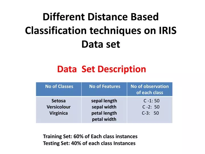
Different Distance Based Classification techniques on IRIS Data set. Data Set Description . Training Set: 60% of Each class instances Testing Set: 40% of each class Instances . Distance Metrics. Euclidean Distance (Squared ED, Normalized Square ED)

E N D
Different Distance Based Classification techniques on IRIS Data set Data Set Description Training Set: 60% of Each class instances Testing Set: 40% of each class Instances
Distance Metrics • Euclidean Distance (Squared ED, Normalized Square ED) • City Block Distance (=Manhattan Distance) • Chess Board Distance • Mahalanobis Distance • Minkowski Distance • Chebyshev Distance • Correlation Distance • Cosine Distance • Bray-Curtis Distance • Canberra Distance
Vector Representation 2D Euclidean Space
Properties of Metric Triangular Inequality 1). Distance is not negative number. 2) . Distance can be zero or greater than zero.
Classification Approaches Generalized Distance Metric • Step 1: Find the average between all the points in training class Ck . • Step 2: Repeat this process for all the class k • Step 3: Find the Euclidean distance/City Block/ Chess Board between Centroid of each training classes and all the samples of the test class using • Step 4: Find the class with minimum distance.
Mahalanobis Distance is the covariance matrix of the input data X B When the covariance matrix is identity Matrix, the mahalanobis distance is the same as the Euclidean distance. Useful for detecting outliers. A P For red points, the Euclidean distance is 14.7, Mahalanobis distance is 6.
Mahalanobis Distance Covariance Matrix: C A: (0.5, 0.5) B: (0, 1) C: (1.5, 1.5) Mahal(A,B) = 5 Mahal(A,C) = 4 B A
City Block Distance City Block Distance
Geometric Representations of City Block Distance City-block distance (= Manhattan distance) The dotted lines in the figure are the distances (a1-b1), (a2-b2), (a3-b3), (a4-b4) and (a5-b5)
Chess Board Distance Euclidean Distance City Block Distance Chess Board Distance
Correlation Distance • Correlation Distance [u, v]. Gives the correlation coefficient distance between vectors u and v. Correlation Distance [{a, b, c}, {x, y, z}]; u = {a, b, c}; v = {x, y, z}; CD = 1 - (u – Mean [u]).(v – Mean [v]) / (Norm[u - Mean[u]] Norm[v - Mean[v]])
Cosine Distance Cosine distance [u, v]; Gives the angular cosine distance between vectors u and v. • Cosine distance between two vectors: Cosine Distance [{a, b, c}, {x, y, z}] CoD = 1 - {a, b, c}.{x, y, z}/(Norm[{a, b, c}] Norm[{x, y, z}])
Bray Curtis Distance • Bray Curtis Distance [u, v]; Gives the Bray-Curtis distance between vectors u and v. • Bray-Curtis distance between two vectors: Bray-Curtis Distance[{a, b, c}, {x, y, z}] BCD: Total[Abs[{a, b, c} - {x, y, z}]]/Total[Abs[{a, b, c} + {x, y, z}]]
Canberra Distance • Canberra Distance[u, v]Gives the Canberra distance between vectors u and v. • Canberra distance between two vectors: Canberra Distance[{a, b, c}, {x, y, z}] CAD: Total[Abs[{a, b, c} - {x, y, z}]/(Abs[{a, b, c}] + Abs[{x, y, z}])]
Minkowski distance • The Minkowski distance can be considered as a generalization of both the Euclidean distance and the Manhattan Distance.
Output to be shown • Error Plot (Classifier Vs Misclassification error rates) • MER = 1 – (no of samples correctly classified)/(Total no of test samples) • Compute mean error, mean squared error (mse), mean absolute error