Download
1 / 19
190 likes | 397 Views
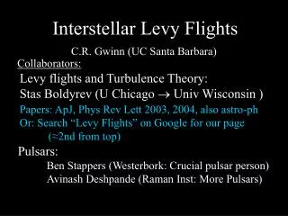
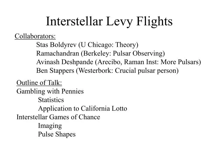
Interstellar Levy Flights. Collaborators: Stas Boldyrev (U Chicago: Theory) Ramachandran (Berkeley: Pulsar Observing) Avinash Deshpande (Arecibo, Raman Inst: More Pulsars) Ben Stappers (Westerbork: Crucial pulsar person). Outline of Talk: Gambling with Pennies Statistics

E N D
Interstellar Levy Flights Collaborators: Stas Boldyrev (U Chicago: Theory) Ramachandran (Berkeley: Pulsar Observing) Avinash Deshpande (Arecibo, Raman Inst: More Pulsars) Ben Stappers (Westerbork: Crucial pulsar person) Outline of Talk: Gambling with Pennies Statistics Application to California Lotto Interstellar Games of Chance Imaging Pulse Shapes
“Gauss” You are given 1¢ Flip 1¢: win another 1¢ each time it comes up “heads” Play 100 flips “Cauchy” You are given 2¢ Flip 1¢: double your winnings each time it comes up “heads” You must walk away (keep winnings) when it comes up “tails” (100 flips max) Gamble and Win in Either Game! Value = ∑ Probability($$)($$) = $0.50 … for both games Note: for Cauchy, > $0.25 of “Value” is from payoffs larger than the US Debt.
“Core” The resulting distributions are then approximately Gaussian or Cauchy (=Lorentzian) “Halo” or “Tail” Symmetrize the Games Gauss: lose 1¢ for each “tails” Cauchy: double your loss each “tails” -- until you flip “heads”
Play Either Game Many Times The distributions of net outcomes will approach Levy stable distributions. “Levy Stable” => when convolved with itself, produces a scaled copy. In 1D, stable distributions take the form: P b($)=∫ dk ei k ($) e-|k| Gauss will approach a Gaussian distribution b=2 Cauchy will approach a Cauchy distribution b=1
The Central Limit Theorem says: the outcome will be drawn from a Gaussian distribution, centered at N$0.50, with variance given by…. To reach that limit with ”Cauchy”, you must play enough times to win the top prize. Fine Print …and win it many times (>>1033) plays.
California Lotto Looks Like Levy • Prizes are distributed geometrically • Probability~1/($$) • Top prize dominates all moments: ∑ Probability($$)($$)N≈(Top $)N
Does it matter which we choose? Are there observable effects? Are there media where Cauchy is true? Do observations tell us about the medium? Isn’t this talk about insterstellar travel? When waves travel through random media,do they choose deflection angles via Gauss or Cauchy? • People have worked on waves in random media since the 60’s, (nearly) always assuming Gauss.
Interstellar Scattering of Radio Waves • Long distances (pc-kpc: 1020-1023 cm) • Small angular deflection (mas: 10-9 rad) • Deflection via fluctuations in density of free electrons (interstellar turbulence?) • Close connections to: • Atmospheric “seeing” • Ocean acoustic propagation
3 Observable Consequencesfor Gauss vs Cauchy • Shape of a scattered image (“Desai paradox”) • Shape of a scattered pulse (“Williamson Paradox”) • Scaling of broadening with distance (“Sutton Paradox”)
Let’s Measure the Deflection by Imaging! • At each point along the line of sight, the wave is deflected by a random angle. • Repeated deflections converge to a Levy-stable distribution of scattering angles. • Probability(of deflection angle) –is– the observed image*. • * for a scattered point source. • Observations of a scattered point source should give us the distribution. b=1 b=2 Simulated VLB Observation of Pulsar B1818-04
Excess flux at long baseline: sharp “cusp” Excess flux at short baseline: big “halo” Best-fit Gaussian model *”Rotundate” baseline is scaled to account for elongation of the source (=anisotropic scattering). It Has Already Been Done Desai & Fey (2001) found that images of heavily-scattered sources in Cygnus did not resemble Gaussian distributions: they had a “cusp” and a “halo”. Actually, radio interferometry measures the Fourier transform of the image -- usually confusing -- but convenient for Levy distributions! Intrinsic structure of these complicated sources might create a “halo” – but probably not a “core”!
Pulses Broaden as they Travel Through Space Mostly because paths with lots of bends take longer!
The Pulse Broadening Function (Impulse-Response Function) is Different for Gauss and Cauchy For Cauchy, many paths have only small deflections – and some have very large ones – relative to Gauss Dotted line: b=2 Solid line: b =1 Dashed line: b =2/3 (Scaled to the same maximum and width at half-max)
Observed pulses from pulsars tend to have sharper rise and more gradual fall than Gauss would predict. • Williamson (1975) found that models with all the scattering material concentrated into a single screen worked better than models for an extended medium. • Cauchy works at least as well as a thin-screen model -- for cases we’ve tested. Go Cauchy! Solid curve: Best-fit model b=1 Dotted curve: Best-fit model b=2
Is the Problem Solved? • For Cauchy-vs-Gauss-vs-Thin Screen, statistical goodness of fit is about the same • Cauchy predicts a long tail – which wraps around (and around) the pulse – could we detect that? • Or at least unwrap it? Horizontal lines show zero-level
Pulse broadening is greatest at low observing frequency (Because the scattering material is dispersive.) • We fit for pulse shape at high observing frequency, and for degree of broadening at low frequency. • Fits at intermediate frequency (with parameters taken from the extremes) favor Cauchy – though neither fits really well! From Westerbork: Ramachandran, Deshpande, Stappers, Gwinn
We have more nifty ideas Cauchy arrives • The travel time for the peak of a scattered pulse is pretty different for Gauss and Cauchy (sorta like the most common payoff in the games “Gauss” and “Cauchy”) • Without scattering, the pulse would arrive at the same time as the pulse does at high frequency*. • *If we’ve corrected for dispersion. • We can measure that if we do careful pulse timing. Gauss arrives Pulse at 1230 MHz (no one’s keeping track of time) Pulse at 880 MHz
Have we learned anything? • The lottery can be a good investment, depending on circumstances. • But, you are not likely to win the big prize. • The lottery (and more boring games) have much to teach us about wave propagation. • We can tell what game is being played by examining the outcomes carefully.
Levy Flights Fact: If the distribution for the steps has a power-law tail, then the result is not drawn from a Gaussian.It will approach a Levy distribution: P b(Dq)=∫ dk ei k Dq e-|k|P b(Dq) ®Gaussian for b®2Rare, large deflections dominate the path: a “Levy Flight”. b Klafter, Schlesinger, & Zumofen 1995, PhysToday JP Nolan: http://academic2.american.edu/~jpnolan/