Download
1 / 18
200 likes | 447 Views
Quantum simulations: solid state devices. Max-Planck Institut für Quantenoptik Tutorial talk @ Ringberg December, 10 th , 2007 Matteo Rizzi. Outline. 0. Basic motivations: why a q-sim is more feasible than a q-comp? Solid state device I: Josephson Junction Arrays

E N D
Quantum simulations: solid state devices Max-Planck Institut für Quantenoptik Tutorial talk @ Ringberg December, 10th, 2007 Matteo Rizzi
Outline • 0. Basic motivations: why a q-sim is more feasible than a q-comp? • Solid state device I: Josephson Junction Arrays • Quantum phase model definition • Frustration effects • Other implementable models • Experimental techniques (hints) • Solid state device II: Quantum Dot Arrays • Experimental Realization • Fermi Hubbard mapping • Experimental techniques (hints) • Brief comparison with Cold Atoms in Optical Lattices
Quantum Computers will exploit superposition & 2-bit gates to getpolynomial scaling Basic motivations Well known difficulties in Classical Computers (expon. scaling) e.g. 200 spins requires as many coefficients as protons in the universe ! Universal Q-Comp requires 103 bites & 102 ancillas each: will be optimistically feasible in 20 years ! … and not every problem is polynomial (e.g. 2D Hubb spectrum)
Let a system A be well manipulable (both Hamiltonian and states) and its observables readable by experimental protocols. If A matches some mapping to a system B: all the properties of B can be studied and read in A !! R.P. Feynman, Int. J. Theor. Phys. 21, 467 (1982) B can even be a toy model built on pen&paper: Hamiltonian engineering Basics: Shortcut to quantum simulations Liquid NMR 4He (hard-core bosons) SOLID STATE (Josephson Junctions & Quantum dots) Hubbard models (with frustration), Spin models, Dissipation, … Optical lattices Hubbard, Spin, High Tc BEC sound waves Black holes Coupled cavities Dirac equations Ion Traps Cosmological creation
Josephson effect • Phase evolution • El.Magn. gauge invariance • Electrostatic energy • Small junctions, to see quantum Device 1: Josephson Junctions
Typical experimental numbers: • Sjunc = 10-2 mm2 • Sisl = 0.5 mm2 • Splaq = 5 mm2 • F0/plaq = 5 G • Rn = 5-50 KW • C = 1-10 fF C0 = 10-2 fF • Nisl = 105 • Ec, EJ = 10 – 100 meV Inverse capacitance matrix D1: JJ arrays’ definitions
Short range (on-site) Long range (logarithmic) D1 JJAs: Quantum phase model
With long-range charge term • checkerboard Wigner solid ! • Longer range more lobes • Out of it, maybe room also for • a supersolid phase • (i.e. both diag & off-diag order) D1 JJAs: frustration effects (electric)
(more structured geometries) (square) may lead to Aharanov-Bohm insulators Resembling Hofstatter butterfly… D1 JJAs: frustration effects (magnetic) Magnetic frustration:
Quantum Phase Model can be seen as • a “high occupation number” approximation of Bose-Hubbard: • an equivalent XXZ spin ½ Heisenberg chain (strong Coulomb blockade) Both have the same BKT universality class ! (although details may change) D1 JJAs: other models
D1 JJAs: experimental detection Basic technique is current-voltage transport through lattice Much more interesting physics can be done with JJAs: quantized vortices, dissipation effects, some kind of Hall regime, … R. Fazio, H. van der Zant, Phys. Rep. 355 235–334 (2001)
Device 2: Quantum dot arrays T. Byrnes,N.Y. Kim,K. Kusudo,and Y. Yamamoto, arXiv:0711.2841v2 [quant-ph] (dec. 2007) • List of ingredients to get a Fermi-Hubbard simulator • 2DEG at semiconductors inteface • GG global gate to tune population & screen Coulomb • MG mesh gate to get periodic potential • INSulator strip to make GG & MG independent ! • Source S & Drain D to make transport measures
Typical experimental numbers: • Ssample = 30x30mm2 • lMG = 0.1 mm • d2DEG = 30 nm • e2DEG= 13 e0 • m*2DEG = 1/16 me • r2DEG = 1011 cm-2 • nel/QDOT = 10 - avoid density transitions - overcome impurities GG Coulomb screening due to image charges Without GG screening , with it elec.repulsion comparable to hopping D2 QDAs: important features
Standard Wannier (exact) mapping Splitting the on-site term, including intraband correlations… D2 QDAs: Fermi-Hubbard mapping (1) …get a local effective Hamiltonian, and then include site-site terms
Nondegenerate Degenerate (2-fold) • Empirical Hund’s rule holds • effective 2-band Hubbard structure Hopping & n.n. interactions recovered by mapping also onto the effective basis D2 QDAs: Fermi-Hubbard mapping (2) Outer shell is the important one !
V0 = 5.4 meV Interband suppressed Nb < 12 V0 tuned by mesh gate MG, Nb by global gate GG … D2 QDAs: tunability & requirements choosing the right band, and tuning V0 , one should get MI-SF transition AF visible T < 0.1 t // d-wave SC T < 0.02 t T = 10 mK = 1 meV is OK !
Moreover, leads to effective t-J or Heisenberg models and arbitrariety in MeshGate allows for frustrated triangular lattices ! Disorder in mesh pattern leads to Hubbard-Anderson model D2 QDAs: exp. detection & models Cooper pairs Magn.Capac. Oscill. Period AF nature T-varying Magn.Suscept. Scaling theory of quantities even far from QPT Phase-breaking length Magnetoconductance Any other kind of transport property btw. Source & Drain