Download
1 / 48
480 likes | 631 Views
NACP. GC51G-02. Towards validation of urban GHG emissions using a very high resolution atmospheric inversion in the Indianapolis Flux Experiment.

E N D
NACP GC51G-02 Towards validation of urban GHG emissions using a very high resolution atmospheric inversion in the Indianapolis Flux Experiment Kenneth J. Davis1, Thomas Lauvaux1, Laura E. McGowan1, Maria Cambaliza2, Michael Hardesty3, Laura T. Iraci4, Kevin R. Gurney5, Patrick W. Hillyard4, Anna Karion3, Natasha L. Miles1, James R. Podolske4, Igor Razlivanov5, Scott J. Richardson1, Daniel P. Sarmiento1, Paul B. Shepson2, Yang Song5, Colm Sweeney2, Jocelyn Turnbull6, James Whetstone7 1The Pennsylvania State University, 2Purdue University, 3NOAA ESRL, 4NASA Ames, 5Arizona State University, 6GNS Science, 7NIST AGU Fall Meeting, San Francisco, CA, 7 December, 2012
INFLUX Objectives • Test “top-down” and “bottom-up” approaches to urban anthropogenic CO2 and CH4 emissions quantification. • Compare whole-city estimates using three different approaches (inventory, tower inversion, aircraft budget). • Determine GHG emissions at 1 km2 resolution and with 10% precision and accuracy across the city using atmospheric inversions. • Quantify the uncertainty in atmospheric budget and inversion methods at the urban scale
Outline • Inversion system description • Observations! • Forwards modeling • Simulated influence of boundary conditions • Influence of sectoral emissions • (Model-data comparisons) – only qualitative • Atmospheric inversions • System design experiment • (Real data inversions)
Inversion system Not a model! A system for model-data synthesis
Air Parcel wind wind Sinks Air Parcel Air Parcel Sources Sample Sample Tower-based atmospheric inversion system Boundary and initial conditions (GHGs/met): (Carbon Tracker, NOAA aircraft profiles, NCEP meteorology) Atmospheric transport model: (WRF-chem, 1-2 km) Prior flux estimate: (Hestia and Vulcan, EDGAR and EPA, CT posterior and/or VPRM) Network of tower-based GHG sensors: (~11-12 sites with CO2, CH4, CO and 14CO2)
Inversion system, continued • Lagragian Particle Dispersion Model (LPDM, Uliasz). • Determines “influence function” – the areas that contribute to GHG concentrations at measurement points.
Inversion system NOAA aircraft, boundary towers Lateral boundary CO2 x0 B H Purdue aircraft campaign Flux tower sites Estimated together R x WRF vs LPDM Hx0 y y-Hx0 Instrument error Uncertainties (flux and observational) estimates from model-data comparisons in the study region. (following Lauvaux et al., 2012, ACPD)
Modifications for INFLUX • Urban boundary layer and land surface simulated (well?) in WRF-Chem. Evaluate with meteorological observations. • CO/CO2/14CO2 incorporated to disaggregate fossil and biogenic CO2. (A31H-02: Turnbull) • Strong, relatively well-known point sources quantified prior to regional inversion. • power plant – CO2 • landfill, waste water treatment plant – CH4
Observations GC53B-1279: Cambaliza GC53B-1284: Miles
Picarro, CRDS sensors; NOAA automated flask samplers; Communications towers ~100m AGL INFLUX ground-based instrumentation GC53B-1284: Miles
Status of ground-based observational system • 9 GHG towers installed and running (1 to be moved, 3 more to be installed ASAP). • 1 flux system installed, 3 more in prep. • Doppler lidar scheduled for installation this winter. • TCCON to be removed next week. Deployment and operation of a network like this is a large effort. Use our data!
Observed: Comparison of [CO2] at 8 INFLUX sitesSeptember – November 2012. • [CO2] at 3 pm local at 8 sites in the Indianapolis area • Synoptic-scale variability in [CO2] is apparent 15 Sept 15 Oct 15 Nov 2012 * Note: Tower heights range from 40 m AGL to 136 m AGL
Observed: Comparison of [CO2] at 8 INFLUX sites September – November 2012 • [CO2] at 3 pm local at 8 sites, with 15-day smoothing (removes most of the weather-driven variability) 15 Sept 15 Oct 15 Nov 2012 * Note: Tower heights range from 40 m AGL to 136 m AGL
Observed: Comparison of [CO2] at 8 INFLUX sites September – November 2012 • Site 03 (downtown) is consistently higher than the other sites. • Site 09 (background site to the east of the city) measures the lowest average [CO2] * Note: Tower heights range from 40 m AGL to 136 m AGL
Picarro, CRDS sensors; NOAA automated flask samplers; Communications towers ~100m AGL INFLUX ground-based instrumentation GC53B-1284: Miles
Observed: Dependence of CO2 spatial gradient on wind speed • 15 Nov 2012 at 3 pm local • Winds: calm Light winds: 15 ppm difference midday
Observed: Dependence of CO2 spatial gradient on wind speed • 12 Nov 2012 at 3 pm local • Winds: 9 m/s from the west Strong winds: < 2 ppm difference midday
CH4 Enhancement (Site 02 – Site 01) as a Function of Wind Direction April – November 2011 (Afternoon hours only) Note the LARGE day to day variability!
CH4 Enhancement (Site 02 – Site 01) as a Function of Wind Direction April – November 2011 (Afternoon hours only) N • Green arrows point to the source for enhancements measured at Site 02, whereas the black arrows point to the source for enhancements measured at Site 01 • In addition to the known source to the southeast of Site 02, there is an additional source to the southwest of the city. CH4 enhancement 10 5 W E S
Picarro, CRDS sensors; NOAA automated flask samplers; Communications towers ~100m AGL INFLUX ground-based instrumentation GC53B-1284: Miles
CO2 Enhancement (Site 02 – Site 01) as a Function of Wind Direction
CO2 Enhancement (Site 02 – Site 01) as a Function of Wind Direction April – November 2011 (Afternoon hours only)
CO Is the CO enhancement reduced when the wind is from the power plant?
TCCON vs in-situ comparison: CH4 Are the residuals indicative of variability in Free Tropopsheric mole fractions?
Status of modeling system • WRF-Chem running with: • 3 nested domains, inner domain 1km2 resolution, 87x87 km2 domain • Meteorological data assimilation • Hestia anthropogenic fluxes for the inner domain • Vulcan anthropogenic fluxes for the outer domains • Carbon Tracker posterior biogenic fluxes • Carbon Tracker boundary conditions
Status of modeling system • LDPM influence functions computed for Oct 7th – Nov 10th, 2011 and 3 flights in 2011. • “Forward” simulations for Oct 7th – Nov 10th, 2011 and 5 flights in 2011 with: • Hestia emissions to examine sectoral CO2 influences at various towers (but simple boundary conditions and no biogenic fluxes). • Vulcan emissions with CT biogenic fluxes and lateral boundary conditions • Inversion system test, neglecting influence of lateral boundary conditions and biogenic fluxes • (Real data inversion) – not yet
Status of modeling system • Model-data comparisons • Case studies of vertical mixing, plume dispersion – last AGU • (Comparison of long-term patterns in GHG mixing ratios) - qualitative • (Long-term evaluation of meteorological performance) - pending • (Comparisons of flight data to atmospheric simulations) - pending
Outer domain Vulcan emissions Vulcan emissions cropped – Hestia within inner domain
Can we detect anthropogenic emissions? Or do biogenic fluxes and lateral boundary conditions dominate?
Winter CO2 differences, tower 2 vs. 1 Total CO2 difference Each point is 20 minutes. 10 day sequence. Midday data. Includes full suite of boundary conditions and biogenic fluxes. Note drop with wind speed. Mole fraction (ppm)
Winter CO2 differences, tower 2 vs. 1: Broken down by source of CO2 Anthropogenic within domain fluxes, 10 ppm scale Biogenic within domain fluxes, 0.5 ppm scale Total boundary condition inflow, 12 ppm scale • Tentative conclusion: • Inflow is of similar magnitude to Indy anthro fluxes. • Similar conclusion for bio fluxes in summer?
Inversion system test • 6 tower system tested, hourly daytime data • Prior fluxes with and without strong point sources • Prior errors proportional to fluxes • Prior error correlations 3km, isotropic, correlated with land cover • Noise added with same spatial statistics, 80% of flux magnitude • 7 day Bayesian matrix inversion, November • No biogenic fluxes, no boundary conditions
Hestia total emissions without point sources Flux units: gC m-2 hr-1. Point sources need special treatment
Prior emissions errors Standard deviation = 80% of flux Flux units: gC m-2 hr-1.
Sample of influence functions for 6 towers Particle touchdown for July 12, 2011 after a) 12 hours and b) 72 hours. Touchdown is considered within 50m of surface. The background values are EPA 4km CO.
Gain – relative improvement prior vs. posterior Very good system performance within the tower array. Very idealized case, but encouraging nonetheless. 1 = perfect correction to prior fluxes Flux units: gC m-2 hr-1.
Hestia emissions in the atmosphere Can we isolate fluxes from individual emission sectors?
Hestia sectoral emissions within the inner domain Residential sector Road sector Industrial sector Commercial sector
Hestia sectoral emission atmospheric mole fractions Mixing ratios of tenths to a few ppm Residential sector [CO2] Oct 8th 17:00LT Road sector Industrial sector Commercial sector
Sectoral atmospheric mole fractions, tower by tower Winter mean mole fractions 6 of 12 tower sites Midday ABL mixing ratio (ppm) Site 1: background Site 2: downwind Site 10: powerplant! Small mixing ratios(?) Some structure across towers by sector. Site 1 Site 10 2 5 9 7 commer indust mobile resid powerplant
Picarro, CRDS sensors; NOAA automated flask samplers; Communications towers ~100m AGL INFLUX ground-based instrumentation GC53B-1284: Miles
Conclusions • Tower observations detect a clear urban signal in both CO2 and CH4 (buried amid lots of synoptic “noise”). • Simulations suggest thatlateral boundary conditions (and biogenic fluxes?) are of similar magnitude to urban emissions in determining tower-tower differences in CO2. • Inversion system with 6 towers performs very well under idealized conditions. • Sector contributions are likely difficult to identify from tower CO2 alone.