Download
1 / 63
861 likes | 1.69k Views
Static Magnetic Fields. Simple observations Biot-Savart Law & Examples Ampere’s Law & Examples Ampere’s Law in point form The Curl Stoke’s Theorem & Examples Maxwell’s Equations for Static Fields Magnetic Vector Potential. Experimental - Magnetic Forces Between Currents.

E N D
Static Magnetic Fields • Simple observations • Biot-Savart Law & Examples • Ampere’s Law & Examples • Ampere’s Law in point form • The Curl • Stoke’s Theorem & Examples • Maxwell’s Equations for Static Fields • Magnetic Vector Potential
Experimental - Magnetic Forces Between Currents Magnetic forces arise from charges in motion. Forces between current-carrying wires help determine what magnetic force field should look like: 3 easily-observed situations: • How do we describe field around wire 1 that can be used to determine force on wire 2? • “Fields” (like E field) break the problem into two parts.
The Magnetic Field Wire 1 creates field H which circulates around 1 by Right-Hand Rule 1 (Right thumb in direction of current, fingers curl in direction of H) Wire 2 interacts with field H to produce force by Right-Hand Rule 2 (Hand in direction I2, then H, thumb points in direction of force) • Examine 3 cases: • I1 up, I2 up, force attractive • I1 up, I2 down, force repulsive • I1 up, I2 into plane, no force • Note B = H in free space, similar to D =εoE.
Magnetic field contribution dHcreated by “point source” current element dL. Units H are [A/m] • Note • Inverse-square distance dependence • Cross product yields vector pointing into page • Similarity with Coulomb’s Law >> Biot-Savart Law
At point P, the magnetic field from differential current element IdLis To determine total field at P from closed circuit path, sum contributions from current elements over entire loop Magnetic Field From Complete Current Loop
Example 1 - H around Long Wire Evaluate magnetic field H on y axis (or xyplane) from infinite current filament along z axis. Vector from source to observation point: Unit vector from source to observation point: Biot-Savart becomes: (into page by RHR)
Example 1 - H around Long Wire II Integrating over entire wire: Using cross products
Current into page. • Magnetic field streamlines • concentric circles • decrease with inverse distance from the z axis Example 1 – H around Long Wire III End view of wire Ampere’s law near long wire
Example 2 - H from Finite Current Segment Field is found in xyplane at Point 2. Biot-Savart integral is taken over finite wire length: Which simplifies to (Problem 7.8):
Example 3 – H for right-angle segments e.g. motor winding?
Biot-SavartLaw: Example 4 - H from Current Loop Vector from source to observation point: Current length element:
Substituting R and ar in Biot-Savart Law: Carrying out cross products: Substitute for of angular-dependent radial unit vector: radial components not integrate to zero, only z-component remains. Example 4 - H from Current Loop II
Only z component remains, integral evaluates to: Numerator is product of current and loop area. We define magnetic moment as: Example 4 - H from Current Loop III
For surface carrying uniform current density K [A/m], current within width b is: So the differential current quantity is: And Biot-Savart law over 2D surface is: And Biot-Savart law over 3D surface (plus depth) is: Two- and Three-Dimensional Currents
Ampere’s Circuital Law states that the line integral of H around any closed path is equal to the current enclosed by that path. Line integral of H around closed paths a and b gives total current I, integral over path c only gives portion of current that lies within c Practical use requires knowledge of symmetry of path Ampere’s Circuital Law
Example 1 - Ampere’s Law Applied to Long Wire Symmetry suggests H will be circular, constant-valued at constant radius, and centered on current (z) axis. Choosing path a, and integrating H around circle of radius gives enclosed current,I: Same as Biot-Savart Law.
Two concentric conductors carry equal and opposite currents, I. Line assumed to be infinitely long, and circular symmetry suggests H will be entirely - directed, and vary only with radius . Example 2 - Ampere’s Law for Coaxial Transmission Line • Four Regions • Field within inner conductor • Field between conductors (same as long wire) • Field within outer conductor • Field outside both conductors (zero, since net enclosed current zero)
Current distributed uniformly inside conductors, the H assumed circular everywhere. Ampere’s Law inside inner conductor at radius : Current enclosed is Combining Example 2 - Field Within Inner Conductor
a < < b Example 2 - Field between Conductors As with long straight wire: Result:
Inside outer conductor, the enclosed current consists of the inner conductor current plus that portion of the outer conductor current at radii less than Ampere’s Circuital Law becomes So H is: Example 2 - Field Inside Outer Conductor
Outside the transmission line no current is enclosed by the integration path, so 0 The current is uniform with circular symmetry over the integration path, and thus must be 0: Example 2 - Field Outside Both Conductors Applications: Coaxial line (Twisted pair)
Combining previous results, and assigning dimensions as in the inset below: Example 2 - Field over entire Radius of Coax Line
Uniform plane current in y direction, H should be x-directed from RHR and symmetry. • No Hy in direction of current (RHR) • No Hz since overlapping filament components cancel (RHR) • Applying Ampere’s Law to path 1 - 1’ – 2 - 2’. Thus magnetic field is discontinuous across current sheet by magnitude of the surface current density. Example 3 - Ampere’s Law for Current Sheet
If loop 1 – 1’ – 3 – 3’ is outside current plane: 1. By symmetry, field magnitude above sheet must be same as field magnitude below sheet 2. Also from previous page: so field is constant outside current plane Example 3 - Ampere’s Law for Current Sheet II Combining 1 and 2 Half the magnetic field / surface current discontinuity is on each side of the current sheet.
Magnetic field above current sheet is equal and opposite to field below sheet. Field in either region written as cross product: where aNis unit vector normal to current sheet, and points into region where field is evaluated. Example 3 - Ampere’s Law for Current Sheet III
Applying Ampere’s Law to rectangular path Δz long through side of solenoid: Where paths DA and BC are radially in and out, and CD is parallel at a great distance. N/d is number of turns per/length. Example 4 - Ampere’s Law for Solenoid
Paths BC and DA are oppositely-directed and cancel, and path CD is evaluated at great distance where H is zero. Example 4 - Ampere’s Law for Solenoid II Where N/d is number of turns per/length, and (N/d)IΔz is the total current through the path. The field is thus
A toroid is a doughnut-shaped set of windings around a core material. A cross-section with inner radius (ρo – a) and outer radius (ρo+ a) is shown below. The windings are modeled as N individual current loops, each of which carries current I Example 5 - Ampere’s Law for Toroid
Ampere’s Law is applied by taking a line integral around the circular path Cat radius By symmetry His assumed to be circular and a function of radius only: Ampere’s Law takes the form: Result: Performing line integrals in regions ρ < (ρo - a) and ρ> (ρo+ a) enclose no net current, and lead to no magnetic field Example 5 - Ampere’s Law for Toroid II
Ampere’s Law in Point Form Consider magnetic field H at center of a small closed loop. We approximate field over closed path 1-2-3-4 by extrapolating H to each of 4 sides. This will be the point form of Ampere’s Law
Line Integral H∙ΔL Along Front Segment Line integral along front segment 1-2: Extrapolating H to front segment: How the y component is changing as you move in the x direction shear Combining 2 terms:
Line Integrals along Front and Back Segments The contribution from front side 1-2 is: The contribution from back side 3-4 is: Note signs used in extrapolating H to front and back, and in evaluating line integral direction.
Line Integrals along Side Segments The contribution from right side 2-3: The contribution from left side 4-1: Note signs used in extrapolating H to right and left, and in evaluating line integral direction.
Line Integral from entire Closed Loop The total integral is now the sum: Combining previous results:
Entire Line Integral related to Current Density Complete line integral now equated to total current passing through loop in z direction JzΔxΔy by by Ampere’s Law. Dividing by loop area gives: Expression becomes exact as Δx, Δy → 0
Similar results can be obtained with the rectangular loop in the other two orthogonal orientations: Loop in yz plane: Loop in xz plane: Loop in xy plane: This gives all three components of current density field. Line Integral in Other Loop Orientations
Using the Definition of the Curl operator This is Ampere’s Circuital Law in point form. (for static fields) Ampere’s Law in Point Form Adding all 3 components and loop orientations
Curl in Rectangular Coordinates Assembling the results of the rectangular loop integration exercise, we find the vector field that comprises curl H: An easy way to calculate this is to evaluate the following determinant: which we see is equivalent to the cross product of the del operator with the field:
General - Curl of Vector Field In general, curl of vector field is another field normal to original field. The curl component in the direction N, normal to the plane of the integration loop is: Direction of N uses right-hand rule: With right-hand fingers oriented in direction of path integral, thumb points in the direction of normal (the curl).
Curl in Other Coordinate Systems Cylindrical coordinates Spherical coordinates
2 of 4 Maxwell’s Equations • Gauss’s Law • Ampere’s Law • http://en.wikipedia.org/wiki/Maxwell's_equations (static fields)
Consider placing a small “paddle wheel” in a flowing stream of water, as shown below. The wheel axis points into the screen, and the water velocity decreases with increasing depth. The wheel will rotate clockwise, and give a curl component that points into the screen (right-hand rule). Positioning the wheel at all three orthogonal orientations yields measurements of all 3 components of curl. Note the curl is directed normal to both the field and the direction of its variation. Visualization of Curl
Surface S is partitioned into sub-regions, each of small area ΔS Line integral around each ΔS is: Stoke’sTheorem - Add Individual Curls Summing path integrals and curls:
Add curl contributions from all ΔS elements, and note adjacent path integrals cancel! Cancellation here: only contribution to overall path integral is around outer periphery of surface S. . No cancellation here: Stoke’s Theorem – Cancel Internal Paths This is path integral of H over outer perimeter as interior paths cancel This is integral of curl of H over surface S Result is Stoke’sTheorem
Summary - Two Theorems Stoke’s Theorem – Chapter 7 Line integral = Surface integral(Curl) Divergence Theorem – Chapter 3 Surface integral = Volume integral(Divergence) A divergence is a 3d volume derivative going between opposite surfaces, a curl is a 2d shear derivative going around a circle
Example 1 – Stoke’sCalculation II 2nd and 5th curl term zero, as no HΘ 6th term zero, as Hr does not involve Θ Only 1st, 3rd, and 4th remain
Begin with Ampere’s Law in point form (static fields): Integrate both sides over surface S: Left and right equal by Stokes’ Theorem. The center term is just net current through surface S. Equating to the middle Example 2 – Ampere’s Integral Form
Already know for static electric field: Integrand must be zero: (static fields) Thus conservative field has zero curl. Example 3 - 3rd Maxwell’s Equation Using Stoke’s Theorem: Note: when is added to right hand side, this becomes Faraday Induction!