Download
1 / 59
590 likes | 695 Views
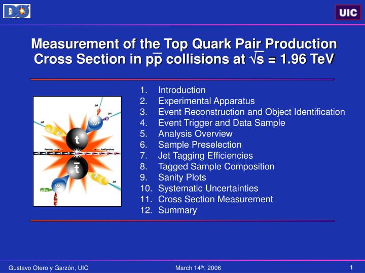
Measurement of the Top Quark Pair Production Cross Section in pp collisions at s = 1.96 TeV. Introduction Experimental Apparatus Event Reconstruction and Object Identification Event Trigger and Data Sample Analysis Overview Sample Preselection Jet Tagging Efficiencies

E N D
Measurement of the Top Quark Pair Production Cross Section in pp collisions at s = 1.96 TeV Introduction Experimental Apparatus Event Reconstruction and Object Identification Event Trigger and Data Sample Analysis Overview Sample Preselection Jet Tagging Efficiencies Tagged Sample Composition Sanity Plots Systematic Uncertainties Cross Section Measurement Summary
Gravitation (10-43) u c t G g strong (1) quarks d s b W weak (10-6) Z e leptons e electromagnetic (10-2) H mass 2nd 3rd 1st What are things made of? All current knowledge of elementary particles and their interactions is condensed in the Standard Model (SM) of elementary particles.
QCD (Strong) Electro-weak (Weak & Electromagnetic) The Standard Model (1) • Quantum Field Theory built on SU(3)xSU(2)xU(1) symmetry • Symmetry conditions on quantum fields gives rise to mediating gauge bosons • Quantum Chromo Dynamics: Strong Interaction • Mediated by gluons (g) carrying two of the three color charges (red, green, blue) • Quarks carry one color charge • Gluons interact with quarks and themselves (non-abelian QFT) • At large distances strong interactions become large: confinement • At small distances strong interactions become small: asymptotic freedom
The Standard Model (2) • Electroweak: QFT combining EM and Weak interactions • Mediated by a photon (g) and weak bosons (W±, Z) • Massless photon infinite range • This theory generates massless particles but: • mW = 80.43 ± 0.04 GeV • mZ = 91.188 ± 0.002 GeV • The mass of the particles is generated by the Higgs Mechanism of Spontaneous Symmetry Breaking, mediated by the Higgs boson (not observed yet) • The SM Lagrangian has 19 free parameters and can be expressed as: LSM = LGauge + LMatter + LHiggs + LYukawa
Why study the Top Quark? • Predicted in the’70s by the SM and discovered in 1995 • Least well studied component of the SM (only produced at the Tevatron so far) • Only known fermion with a mass at the natural Electroweak scale • Lifetime (5x10-25 s) shorter than the hadronization time (no top hadronic bound states) • The top quark is relevant for many Electroweak analyses • Strongest coupling to the Higgs (Yukawa coupling lt mt~ 1)
The Top Quark and the SM Higgs Corrections to W and Z boson masses from top quark and Higgs boson loops constrain the Higgs boson mass MW2 = MW(0) x(1- D) Dt-1 ~ Mt2 Goal for Tevatron in Run II: DMt = 3 GeV DMW = 20 MeV DH ~ ln ( MH2 )
Top Quark Physics W Helicity Production Cross Section Production Kinematics Top Spin Polarization Resonance Production Top Charge Branching Ratios |Vtb| Spin Correlation Non-SM decays Top Mass
Importance of stt • Test Standard Model Predictions • New measurement at a different center of mass energy • Increased statistics (precision measurement) • First step toward any Top property analysis • Process potentially sensitive to New Physics • New heavy resonance • Non-SM contamination in its production and/or decay • These events are an important background source for other physics processes • Single Top • Higgs search • Help improve QCD understanding in preparation for LHC
LHC Tevatron Top Quark Pair Production Top quarks are mainly produced in pairs (through strong interactions) at Tevatron energies • sinel / sttbar~ 1010 • High luminosity • High efficiency
l+jets Top Quark Decay • Top quark decays via the Weak interaction exclusively as t W b • |Vtb|>0.999 • R = 1.03 ± 0.19 (hep-ex/0603002) • Negligible rates for FCNC (t q ,Z,g) • tSM 1.5 GeV (mt=175 GeV) ~10-25 s no hadronic bound states • Final state determined by the decay of the W boson: • dilepton channel (BR ~ 5%, low background) • lepton + jets channel (BR ~ 30%, moderate background) • all hadronic channel (BR ~ 46%, huge background)
signal q' q W ( l ) + 4 jets nµ µ W+ - p p q q' µ nµ b W+ QCD Multijet • fake isolated lepton • misreconstructed MET - t p p - t - q' - W - b p q p q q' b µ - b µ The Lepton + Jets Channel Background • 1 isolated high pT lepton (µ, e) • 1 n(reconstructed as missing transverse energy (MET)) • 4 jets
Introduction Experimental Apparatus Event Reconstruction and Object Identification Event Trigger and Data Sample Analysis overview Sample Preselection Jet Tagging Efficiencies Tagged Sample Composition Sanity Plots Systematic Uncertainties Cross Section Measurement Summary
Right here, right now `p p 1.96 TeV Booster CDF DØ P Tevatron `p `p source Main Injector & Recycler The Tevatron Collider • Proton-antiproton collider with s=1.96 TeV • 36x36 bunches with 396ns between crossings • 3 ~ collisions per bunch crossing • Linst > 1x1032cm-2s-1 • Expected 4-8 fb-1 integrated luminosity for RunII (0.11fb-1 in RunI)
DØ Detector + three tiered trigger system (Event rate reduction from 1.7 MHz to 50 Hz, 200 kB/event)
Introduction Experimental Apparatus Event Reconstruction and Object Identification Event Trigger and Data Sample Analysis Overview Sample Preselection Jet Tagging Efficiencies Tagged Sample Composition Sanity Plots Systematic Uncertainties Cross Section Measurement Summary
Reconstructed objects • Charged Tracks • Primary Vertices • Muons • Electrons • Jets • b-jets • MET Event Reconstruction
Quarks hadronize into jets of particles (extended energy depositions in the hadronic part of the calorimeter) Neutrinos are inferred from energy balance in the transverse plane Electrons are narrow energy depositions in the EM calorimeter with an associated track Muons are reconstructed from hits in the muon system with an associated central track and isolated from calorimeter energy
b-tagging • b-quarks hadronize into long lived (ct~ 450mm) B mesons which travel a few millimeters before decaying • b-jets can be identified! • Soft Lepton Tagging: lepton within a jet from a semileptonic B hadron decay • Lifetime Tagging: tracks significantly displaced from the PV originating from long lifetime of B hadrons
Use of tracks with significant impact parameter with respect to the Primary Vertex • Build-up method fitting pairs of selected tracks within track-jets • Removes track pairs in the mass windows corresponding to K0S, L0 and photon conversions (g→ e+e-) Secondary Vertex Tagger Algorithm The Secondary Vertex Tagger (SVT) is a lifetime tagger that explicitly reconstructs vertices which are displaced from the Primary Vertex • A jet is identified as a b-jet (tagged) if it contains a reconstructed secondary vertex within a jet Top events have two b-jets while events from other processes very seldom have heavy flavor!
Introduction Experimental Apparatus Event Reconstruction and Object Identification Event Trigger and Data Sample Analysis Overview Sample Preselection Jet Tagging Efficiencies Tagged Sample Composition Sanity Plots Systematic Uncertainties Cross Section Measurement Summary
Data set used for this analysis Integrated Luminosity L xs N
Event Trigger • The Tevatron delivers a lot of data: = 1033cm-2s-1 X10-25cm2 = 108 s-1 Ntot = Linstx stot • But most of the interesting events rarely occur • The Trigger System is designed to select those interesting events • A lepton and a jet are required at L1, L2 and L3 for this analysis • Trigger efficiencies are measured by folding into the MC the per-object individual trigger conditions observed in data
Precious Data! Data • A fraction of the data delivered by the Tevatron is recorded • Run Quality Selection (all relevant subdetectors working properly) • Luminosity Block Selection (remove short problems during a run) • Event Quality Selection (based on an event-wide variable)
Introduction Experimental Apparatus Event Reconstruction and Object Identification Event Trigger and Data Sample Analysis Overview Sample Preselection Jet Tagging Efficiencies Tagged Sample Composition Sanity Plots Systematic Uncertainties Cross Section Measurement Summary
Analysis Method • Determine the number of selected events for each background • Parameterize the tagging efficiencies determined in data • Determine event tagging probabilities for all the backgrounds • Use the Monte Carlo simulation event kinematics and fold in the tagging efficiencies from data to estimate the number of tagged events • Estimate the ttbar cross section from the excess in the actual number of tagged events with 3 and 4 jets over the background prediction
Introduction Experimental Apparatus Event Reconstruction and Object Identification Event Trigger and Data Sample Analysis Overview Sample Preselection Jet Tagging Efficiencies Tagged Sample Composition Sanity Plots Systematic Uncertainties Cross Section Measurement Summary
ttbar physics bkg QCD preselection b-tagging • All events pass the signal trigger • A tight (loose) isolated lepton • Large MET (neutrino) • At least one jet • MET separated from the lepton in the transverse plane • Second lepton Veto • This is done by requiring Sample Preselection • We are swamped by QCD multijet events • The idea of the preselection is to select a leptonically decaying W boson in association with jets • The aim is to select objects in the final state with high efficiency and purity minimizing the instrumental background
esig efficiency for a loose lepton from a W decay to pass the tight criteria ~85% eQCD rate for a loose lepton in QCD to appear to be tight esig eQCD ~15% Control bins Signal bins Composition of the Preselected Sample • The preselected sample has two main components • Signal and Physics backgrounds • Instrumental background (QCD Multijet with fake lepton and MET) • Determined purely from data by defining two samples (Matrix Method) • Tight sample : the preselected sample ( Nt) • Loose sample : events passing the preselection but with a loose lepton requirement Nl = Nsig + NQCD Nt = esig.Nsig + eQCD.NQCD
Expected number of signal events: Npreselttbar = stheoryttbarxepreselttbarx BR xL • Expected number of non-W background events: Npreseli = stheoryixepreselix BR xL i = single top, diboson (WW, WZ, ZZ) and Ztt Preselection Efficiencies in the e+jets channel • Expected number of W background events: NpreselW = Nsigt - Npreselttbar - S Npreseli Composition of the Preselected Sample • The Matrix Method separates QCD from Physics Backgrounds
Introduction Experimental Apparatus Event Reconstruction and Object Identification Event Trigger and Data Sample Analysis Overview Sample Preselection Jet Tagging Efficiencies Tagged Sample Composition Sanity Plots Systematic Uncertainties Cross Section Measurement Summary
Tagging Efficiencies • The probability for a jet to be tagged is split into: • Probability for a jet to be taggable • Probability for a taggable jet to be tagged • This serves to: • Decouple tagging efficiency from tracking inefficiencies and calorimeter noise problems (absorbed into the taggability) • Compare performance with respect to other taggers • Current versions of MC simulation do not reproduce the observed tagging rates in data • Tagging rates are parameterized in data and applied to the MC
Taggability • A jet is taggable if it has a matched track-jet • Tracks in the track jet must have hits in the Silicon Tracker • Strong dependence on the SMT geometry • Taggability is measured in the preselected lepton+ jets sample • Parameterize vs. hjet and pT jet in 6 bins of PVZ X hjet
b-Tagging Efficiency • b-tagging rate is measured purely from data applying SVT and Soft Lepton Tagger to two samples: • muon-in-jet • muon-in-jet away jet lifetime tagged (enriched in heavy flavor) • Use system8 • Samples with different fractions of signal and background • SVT and SLT have different efficiencies for signal and background • SVT and SLT decorrelated • 8 equations with 8 unknowns • Parameterize in terms of pTjet and hjet
Calibrate MC tagging efficiency for inclusive b(c)-decays Inclusive b-Tagging Efficiency • System8 provides b-tagging efficiency for semimuonic b-decays (ebm) in data • b(c)-tagging efficiency in MC • Measured in ttbar • Matching B-(C) mesons to jets to determine b(c) flavor • Efficiency in MC is artificially higher • Define data-MC semileptonic Scale Factor • Assume that SFb = SFbm
Mistag Rate • A light (u,d,s,g) jet identified as heavy flavor is a mistag (fake tag) • Originated from misreconstruction and resolution effects • Determined from the negative tagging efficiency • Measured in QCD data ( e-data ) • Parameterized vs. pTjet and hjet
Mistag Rate The Negative Tagging Rate is corrected for: • Heavy flavor contamination • Estimated in QCD Monte Carlo • Parameterized vs. pTjet and hjet • Remaining long lived particles (K0s, L0) not present in the negative tagging rate • Estimated in W+jets Monte Carlo • SFll = 1.52 ± 0.03
Introduction Experimental Apparatus Event Reconstruction and Object Identification Event Trigger and Data Sample Analysis Overview Sample Preselection Jet Tagging Efficiencies Tagged Sample Composition Sanity Plots Systematic Uncertainties Cross Section Measurement Summary
Start from the per-jet tagging probability a = b, c, light • Derive event tagging probabilities by weighting each jet in MC with Pa(pT,h) Single tag probability Double tag probability • Take trigger bias into account • Estimate the number of tagged events Event Tagging Probability
Ntagi = Npreseli x Ptagi i = single top, diboson (WW, WZ, ZZ) and Ztt Single Tag Probabilities in the e+jets channel Background Estimate • QCD-multijet production in the tagged sample: • Apply the Matrix Method to the tagged data sample ( esig(qcd) = esig(qcd)tagged ) • Apply QCD tagging probability to the untagged sample • PtagQCD is measured in the ( Nl – Nt) preselected sample • Non-W physics backgrounds:
The dominant background by far W+jets Background • Use the Monte Carlo Simulation • Apply matching procedure of partons from the matrix element generator and reconstructed jets • Rely on ratios of cross-sections of the generated subprocesses (W+light ,W+c,W+cc ,W+b ,W+bb) • W+jets tagging probability contains different contributions
P=1tagtt4j = 0.44 P 2tagstt4j = 0.15 b-Tagging Philosophy • Estimate the ttbar cross-section from observed excess in the number of tagged events with respect to the background prediction • Optimum use of the statistical information (single and double tags)
Introduction Experimental Apparatus Event Reconstruction and Object Identification Event Trigger and Data Sample Analysis Overview Sample Preselection Jet Tagging Efficiencies Tagged Sample Composition Sanity Plots Systematic Uncertainties Cross Section Measurement Summary
Introduction Experimental Apparatus Event Reconstruction and Object Identification Event Trigger and Data Sample Analysis Overview Sample Preselection Jet Tagging Efficiencies Tagged Sample Composition Sanity Plots Systematic Uncertainties Cross Section Measurement Summary
Introduction Experimental Apparatus Event Reconstruction and Object Identification Event Trigger and Data Sample Analysis Overview Sample Preselection Jet Tagging Efficiencies Tagged Sample Composition Sanity Plots Systematic Uncertainties Cross Section Measurement Summary
Observed vs. Predicted Tags Control region Signal region Assume sttbar = 7pb Single tags Double tags
Cross Section Extraction • The ttbar cross-section is calculated combining 8 channels • e + jets and m + jets • Single tags and double tags • = 3 jets and 4 jets • Perform a maximum likelihood fit to the observed number of events
m + jets : sttbar = 6.39 +1.36-1.22 (stat+syst) ± 0.42(lumi) pb e + jets : sttbar = 7.57 +1.46-1.31 (stat+syst) ± 0.49(lumi) pb sttbar = 6.96 +1.07-0.98 (stat+syst) ± 0.45(lumi) pb l + jets : sttbarNLO = 6.77 ± 0.42 pb N. Kidonakis and R. Vogt, Phys. Rev. D 68 (2003) Result