Download
1 / 42
420 likes | 473 Views
2-bunch Aug2009. Start with the SPG-2 nodule, selecting a fresh(?) area for seeking S, if I have the time. Inner side. Outer side. rectangle is scan area for Inner map in slide 5 et. seq. Scalebar = 0.6mm. Fe Ni Mn. The "Co" is derived by empirical decontam from the 10keV map.

E N D
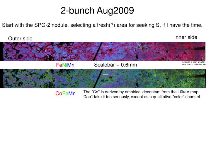
2-bunch Aug2009 Start with the SPG-2 nodule, selecting a fresh(?) area for seeking S, if I have the time. Inner side Outer side rectangle is scan area for Inner map in slide 5 et. seq. Scalebar = 0.6mm FeNiMn The "Co" is derived by empirical decontam from the 10keV map. Don't take it too seriously, except as a qualitative "color" channel. CoFeMn
Compare maps: Outer with long map The long map on slide 1 was done on 8/7, after which came Hoi-Ying's samples (see data/Holman/Aug2009) and a loss-of-position event. Then I came back to the nodule on 8/11 and set up 3 pairs of maps, in Outer, Middle and Inner regions, at 10keV and 4keV, to search for lighter elements. This superposition shows the position discrepancy between the two sets of maps. The green lines show where X and Y take on the values shown in small text in the small map. We see that we're ~300um out in X. Looking at a single feature, I get a discrepancy (Outer_coords-long_coords) of (-279,+33)um. 3000 2000 12500 11500
Outer - light element search SFeMn SKCa ClFeMn K found in Fe-rich matrix, Ca in isolated spots, S in other spots Assuming Cl is a proxy for porosity, we see that the dendritic-looking part is more porous than the Fe-rich matrix that glues it together. This is a bit surprising in that the matrix looks more porous in the maps. Might be worthwhile taking a Cl XANES in the redder parts to make sure that we're really looking at epoxy. Scalebar=0.4mm. S shows in spots containing little Fe,Mn,K,Ca. KFeCu The matrix actually has less Fe than the dendritic Mn-Fe part. Cu, as usual, is streaky.
Middle Scalebar = 0.6mm FeCuNi KFeMn S - not much found ClKCa ClFeMn FeCuNiOuter(same scale as Middle) The Cu/Ni streaks seem proportionatly brighter in Middle than Outer
Inner FeCuNiscalebar = 0.6mm ClKCa KFeMn Cl "Co" ClFeMn Cl seems to be found where "Co" isn't. "Co" is in quotes because it comes from deconamination of FeKb with uncertainty in decontam coeff.
Cu-Ni streaks (Inner) CuNi Ni CuNi masked Cu The streaky part seems to have a consistent Cu-Ni ratio (1.5 Ni counts/Cu count)
Ni-Mn correlation (Inner) In the Ni-Mn scatterplot (left), there's a baseline such that there appears to be a minimum Ni/Mn ratio of about 0.01. Usually, that's leakage from beta or tails. However, if that's the case, then Fe should leak more. The plot on the right shows a baseline slope of about 0.001, 10x less than for Ni. Thus, in the dendritic part (the main bulk of the pixels), there is a consistent Ni/Mn ratio of 1% in counts. This phenomenon is an example of the danger of doing empirical decontamination without a known standard or area in which the element whose channel is to be corrected is known to be absent where the contaminating element is known to exist. Ni vs. Mn Ni vs. Fe
Chem mapping for Ce - Inner Use as a calibrator Ce in our YAG phosphor, which is presumably all 3+. The XANES looks it. I'd rather use CeO2, but I can't find it. The peak for the YAG comes at 5726.0, while the tabulated peaks for the Takahashi 3+ refs (except Ce on Fh) come in at 5725.8. This is insignificantly different, so I'll take the energy scale as good and use 5710, 5726.5, 5738 and 5747 as my energies. As a side note, how important is it to make the V slit narrow? With the slits at 50um and a measured FWHM of 51um, the second moment of the intensity distribution (trucated gaussian) coming through the V slits is the same as that of an un-truncated gaussian of FWHM 31um. Thus, for purposes of broadening, we can think of the FWHM as being 31um. The focal length of M2 is 1300mm, which yields a FWHM broadening of the angular distribution at the mono of 31/1.3= 24urad. At a Bragg angle of 22.4deg (mid-scan) we find a FWHM broadening of 0.3eV, which isn't all that much. It is pretty clear that the narrow slits (red) don't yield much extra detail compared with the wide slits (white). This is due to the low energy (dE ~ E2) and the fact that the L-edge white line is pretty wide.
Energy choices for chem mapping CeO2 Ce-dMnO2 Ce:YAG Ce-Fh 5710 5725.5 5738 5747
Oops! My "background" spots still contain Ce Looks like I'll have to use one.e anyway.
Ce chem map Inner 0.3mm This zoom in of the same map shows the chemical contrast more clearly. No, it isn't color fringing due to drift, since the map-to-map displacements are small.
Glitch cal with CeO2 I found the CeO2 and ran it. A fit to Takahashi's data shows a neglegible energy shift with respect to that standard. Thus, I can use CeO2 for glitch cal.dat as a standard with no E-shift. The glitches are then at 5730.88, 5732.82 (small glitches), 5926.53 and 5933.64 (large glitches). Compare with 5926.00,5934.6 (last tabulation). That the glitches changed spacing shows that we can't describe it just as an energy shift. The smaller glitches should be useful for cal at the V and Ce edges. In order to do this fit, I had to assume that Takahashi's CeO2 was overabsorbed. Of course, the present sample could be overabsorbed as well, but Takahashi's is more so. Takahashi w/ OA=0.2 Present CeO2 1st peak of CeO2 at 5730.39
Distributions The Ce3+ distribution seems to correlate with the Mn and non-streaky part of the Ni distribution. A lineout across a diagonal shows it: Fe Ce3+ Ce3+Mn Ni Ti Mn Ni Ce4+
Distributions The Ce4+ distribution doesn't correlate well with obvious stuff like Fe, Mn, but most closely resembles that of Ca, except for the very bright Ca "rocks" (masked out here). The correlation with Ti looks better on a scatterplot (next slide) or 2D map but isn't obvious in the lineout. Fe Ce3+ Ce4+FeCa Ca Ti Ce4+ Ni
90 10 80 20 Ni 70 30 60 40 50 50 Cu 40 60 30 Zn 70 Mn 20 80 10 90 Ca Fe V Ti Ce 40 30 50 10 60 70 90 20 PCA ITFA on chem map 0 10 90 Ce4+ Ce3+ 20 80 30 70 40 60 2 Mn 0 50 50 From slide 74 Jan2008 RunNotes, Sub_Inner. Vaguely similar. 60 40 Ca 70 Ti 30 Ni 80 20 Fe K 90 10 1 2 Zn Cu 10 80 70 60 50 40 20 90 30 1
Mask off Fe-rich matrix Ce4+FeMn 200mm Ce3+FeMn
Mapping for La According to Takahashi, the La/Ce ratio is an important measure of the Ce anomaly. Thus, we'd like to map both on the same area at the same time. Problem: The V K-edge is <20eV away from the La L3-edge. There are other edges nearby. Thus, it would be hard to separate out the V contribution. Possible solution: Use the LaLb signal at the L2 edge instead. There are no edges of likely elements nearby. A test on a bit of La0.7Sr0.3MnO3 showed the La and Lb to be of nearly equal intensity, but that could be a matrix absorption effect as the sample was thick. Thin-sample relative sensitivity calculation using Mucal: FY cross-section (b/atom) LaLb 0.103 4.18e4 CeLa 0.110 8.07e4 Thus, La would have 48.5% of the sensitivity of Ce. If we assume the nodule to be made of Fe2O3 with a density of 3 (a SWAG), we find an absorption length for the Lab light of 31um, which is about a typical thin-section thickness. The corresponding absorption length for CeLa is about 26um, so not much different. Also, the bin widths for Ce and La are similar (33 vs. 39 channels). Thus, I expect that La will yield half the signal per atom as Ce, and it's highly interfered with, so I don't anticipate the prettiest difference map ever taken. Another problem is that Ce will contribute to the background in the La map.
Data processing 1. DT and resize all 2. Register La+ to La- and Ce+ to Ce- 3. Do differences and make composites including Ti and K channels 4. Register these composites to 10keV 5. Combine all into final composite
Distribution of Lab pixel values The La difference signal is dominated by noise, but the mean is clearly different from 0. The peak at 0 is caused by the masking off of the very bright Ca "rocks" which also show bright in the La channel. Masking off outlying points on the La-Ce scatterplot and taking the average over the whole area of the La and Ce, I get 6144 for the La signal and 96489 for the Ce, for a ratio of 15.7:1. Applying the theoretical sensitivity factor yields a ratio of 7.6:1 (at.). This is clearly above the shale value of 2:1 (wt.). Semilog Linear
Mn XANES on Inner Oct07 This is Brandy Toner's data on the same nodule, but the original Inner region, which is where I first discovered Ce3+. The present region is a few mm above the original. The plot compares the XANES with that of the Manceau standards KBi151 (almost all 4+) and feichtnichite (3+). Except for one point, they're all 4+. Since I see Ce3+ everywhere in Inner, I conclude that it coexists with Mn4+. The heavy lines are the 4+ and 3+ references (white+red). The light lines are the sample.
Mn XANES - closer look Apply overabsorption and energy offset to sample for best match to KBi151 (white). There may be some reduction but not much.
Attempt to quantify V,La,Ce Problem: All 3 of these elements produce fluorescence that falls in similar energy bands. The V K-edge also coincides with the La L3-edge. How to untangle? Try XANES scans over the range including the (VK,La L3),CeL3 and LaL2 edges, with two different ROIs, set to weight the elements differently. Look at the relative edge jumps produced by the elements separately in each of the 6 channels (2 ROIs, 3 edges). Start by making a transect of scans across the nodule and then do standards containing only La (La.7Sr.3MnO3), only Ce (CeO2) and only V (foil). Do a procedure something like "decontamination" to untangle. Here is a table of edge jumps, normalized to the strongest signal: Edge 1st edge 2nd edge 3rd edge 1st edge 2nd edge 3rd edge ROI 470-503 470-503 470-503 492-531 492-531 492-531 SignlName A1 A2 A3 B1 B2 B3 _________________________________________________________________ La 0.502 0 0.607 0.164 0 1 V 1 0 0 0.779 0 0 Ce 0 1 0 0 0.312 0 We see that only Ce contributes to the middle edge, so we can use A2 as the Ce signal. Only La contributes to the 3rd edge, so we use B3 as the La signal. The V signal can then be recovered as A1-0.502*B3, removing La contamination. Problem: The La standard is a thick, absorbing material, and the two peaks are at different incident and exit energies. Therefore, the probe depth will be larger for B3 than A1, thus making that 0.503 factor smaller than it would be for thin samples. Thus, we really have A1=La*x+V; B1=La*y+V*z with x,y,z unknown.
Normalized plots For ROI=470-503, the curve is solid and normalized to go through 1 at the last edge showing. Its partner, 492-531, is shown in dotted with the normalizing factor as the solid. White=La, green=Ce, purple=V
More complications There is lots of Ba in the sample, which makes another edge. The La is tiny compared with V or Ce. That means that the first edge is pretty much all V. Ba Ce V La
Measurement To measure edge jumps. I do linear fits to the regions shown between the lines of like color,. i.e. 5576-5610eV and 5640-5671eV for Ba, and extrapolate to an assumed edge energy in the middle, e.g. 5620eV for Ba. The difference in value between these extrapolations is the edge jump. For Ba and Ce, I use the 470-503 bin, getting the Ba L2 and CeL3 edges, and for La, the 492-531 bin, for the BaL2 edge. This is done with the program Multiscan processor.vi, which automatically reads in the 59 scans, DT's them, regularizes energies, and averages together scans taken at the same positions. 470-503 ch. 492-531 ch. 5660 5710 5780 58700 Ba Ce V 5725 5894 5620 La 5835 5887 5904 5930 5640 5671 5576 5610
Trends over sample Inner Outer BaL2 CeL3 LaL2 There is an overall trend towards low abundance in the Inner region, where Mn is less abundant. Note that the X-axis is reversed from the way it is on maps, which is why Inner is to the left on this graph. This is because the left side of the sample is X+ and the right side X-. X (mm)
Ba-La scatterplot Slope=.053+-.022 r=0.35
Ce-La scatterplot Slope=.028+-.014 r=0.29
Ba-Ce scatterplot Slope=.50+-.23; r=0.29 Remove 2 outliers: Slope=1.17+-0.30; r=0.52
What does this mean for [La]/[Ce]? We see that the counts ratio for La to Ce is about 0.03 based on slope. Summing up all the values from the 58 points yields 0.037. However, the La counts are from the Lb at the L2 edge and the Ce counts from the La at the L3 edge. Referring back to this slide, we see that La should be half as sensitive as Ce. Thus, the atomic ratio is about 0.06-0.075, averaged over the whole transect (Outer to Inner). This does not agree well with the ratio from this slide, derived from difference mapping, of 0.13, but neither is anywhere near the shale value of 0.5.
Valence-state fitting Although the scans weren't designed to probe for valence state, we can see pretty good indications of the oxidation state of the Ce from the ratio of the peaks. I do a pre-edge subtraction in the range 5650-5710eV and post-edge normalization by linear fit in the range 5780-5887. The result is then fit to a sum of Ce:Fh and Ce:MnO2 .e files. Results: Inner Outer
Are the Ce/La ratios different between Inner and Outer? Assume that La is proportional to Ce in both regions. Fit La to a*Ce, with a the unknown. Results: Inner: a=0.016+-.0126 Outer: a=0.039+-.0076 a(Outer)-a(Inner)=0.023+-0.015 (adding error bars in quadrature) Marginal detection of difference.
Bootstrap test There are 14 Inner and 30 Outer points. Randomly assign Inner and Outer Ce-La datapoints to 14-item and 30-item lists. Do the La=a*Ce fits on each list and ask, "what fraction of the time does the difference between the fit coefficients exceed the amount from the real lists"? Here's the code that does that: Answer: The probability of getting the observed difference by chance is 8.0% in 105 trials. This is a 2-tailed test. Thus, at the 90% confidence level, I can say that [La]/[Ce] really is smaller in Inner than Outer. The standard deviation of the difference in fit coefficients is 0.013.
Measurement of contamination matrix Measure contamination coefficients once and for all. Use MicroMatter standards for Fe, Mn to measure, mapping across the plastic ring to get the elastic. Do at popular energies (10,11.5,7,4,14)keV, defining an appropriate elastic+compton channel for each. Also measure Ar->(S,Cl,Si) with no sample at 4keV, S->(Cl,Si) (elemental S sample or rings of Micromatter standards, which contain S) and Cl->(S,Si) (KCl sample). Choice of elastic+compton ROI: E ROI 4 7 FeKb/CoKa 680-734 10 ZnKb 942-996 11.5 1130-1192 (what Pushkar used) 14 1297-1427 For 10keV, use ZnKb default for El+Compt. For 11.5keV, use 1130-1192 (Pushkar). For 7keV, use FeKb/CoKa.
Which is what For Cu,Ni,Fe and Cr,Mn,Ti maps, the scan # vs element+energy table is: # Element E 0 Fe 10 1 Cu 10 2 Ni 10 3 Fe 11.5 4 Cu 11.5 5 Ni 11.5 6 Fe 14 7 Cu 14 8 Ni 14 9 Mn 10 10 Cr 10 11 Ti 10 12 Mn 11.5 13 Cr 11.5 14 Ti 11.5 15 Mn 14 16 Cr 14 17 Ti 14 18 Mn 7 19 Cr 7 20 Ti 7
Light-element maps The sample consisted of tape with S and NH4Cl powders, and a 2mm quartz capillary, partially filled with water and covered with XRF tape a little above where the water ended. The water was there to provide variable elastic scattering. The tape covered up the Si to provide a variable Si signal. Thus, the water part can be used to measure the elastic->X contam coeffs for all but 4keV, and the capillary can be used for Ar->Cl. Identification table: # Sample E ________________________________ 0 Tape on capillary 4 1 Tape on capillary 7 2 Tape on capillary 10 3 Water in capillary 4 4 Water in capillary 7 5 Water in capillary 10 6 Water in capillary 11.5 7 Water in capillary 14 8 NH4Cl 4 9 NH4Cl 7 10 NH4Cl 10 11 NH4Cl 11.5 12 NH4Cl 14 13 S 14 14 S 11.5 15 S 10 16 S 7 17 S 4
Contamination matrix format The contamination coefficients, such that obsCounts[i]=realCounts[i]+T[i,j]*realCounts[j] are to be written into a contamination-matrix file with ctm extension and this format: Lo[0] Hi[0] T[0,0] T[0,1] T[0,2] ... Lo[1] Hi[1] T[1,0] T[1,1] T[1,2] ... ... Note that T[i,j] is the contamination coeff for j->i. Thus, the matrix elements are 0->0 1->0 2->0 0->1 1->1 2->1 ...
14keV Contamination matrix so far. I didn't do K or Ca as contaminants, and should have!