CMAS 10 /11/ 2010 Daven K Henze University of Colorado at Boulder

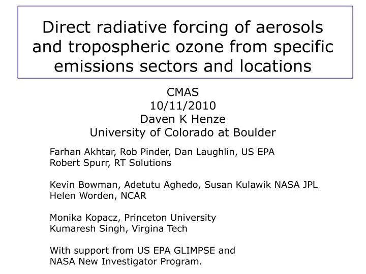
1. Direct radiative forcing of aerosols and tropospheric ozone from specific emissions sectors and locations CMAS 10/11/2010 Daven K Henze University of Colorado at Boulder FarhanAkhtar, Rob Pinder, Dan Laughlin, US EPA Robert Spurr, RT Solutions Kevin Bowman, AdetutuAghedo, Susan Kulawik NASA JPL Helen Worden, NCAR Monika Kopacz, Princeton University Kumaresh Singh, Virgina Tech With support from US EPA GLIMPSE and NASA New Investigator Program.

2. Short Lived Climate Forcing Agents Past: Important for pre-industrial to present radiative forcing Focus on direct effects of - black carbon - sulfate - ozone (trop) AR4, Forster et al., 2007 Future: Addressing SLCFAs important for immediate mitigation efforts as well as air quality.

3. Systems for modeling air quality & climate change

4. Refining the RF bar chart Sector specific contributions: Fuglestvedt et al., 2008 Sector and regional specific contributions: Unger et al., 2008 Unger et al., 2008

5. Systems for modeling air quality & climate change

6. Radiative Forcing Transfer Functions How to calculate the radiative forcing change for a given change in emissions? Using transfer function T:

7. Radiative Forcing Transfer Functions How to calculate the radiative forcing change for a given change in emissions? Using transfer function T: Approximate Tusing adjoint:

8. Aerosols and Radiative Forcing Sensitivities from every sector and region: Calculated very efficiently using GEOS-Chemadjoint (Henze et al., 2007 and LIDORT (Spurr, 2002)

9. Important Approximations Macro - Clear sky - Only direct effects - Only SO4-NO3-NH4-H2O and BC aerosol Micro - Refractive index of SO4-NO3-NH4-H2O is that of SO4. - Assumed dry size - External mixture Conveniance - Only July conditions

10. Radiative Forcing potential The % change in radiative forcing per change in emission: %RF / [kg box] %RF / [kg box] note: per change in any emission. This shows variation in efficiency of emissions forcing.

11. Radiative Forcing sensitivities The sensitivity of pre-industrial to present RF with respect to scaling factors for individual emission sectors Results for different SO2 emissions, Ei,for July 2008: anthropogenic SO2 anthropogen NH3 [%]

12. Radiative Forcing sensitivities The sensitivity of pre-industrial to present RF with respect to scaling factors for individual emission sectors Results for different BC emissions, Ei,for July 2008: biofuel BC fossil fuel BC [%]

13. Applying to global future scenarios: regional and sector-based analysis Consider future CLE scenario for 2030 (Kloster et al., 2008) % of aerosol direct RF (CLE 2030 – present) owing to BC emissions

14. Applying to detailed US scenariossee FarhanAkhtar’s poster Consider estimates of US energy usage from MARKAL Apply RF estimates to BC and SO2 sources WARMING COOLING

15. Validation

16. Radiativeforcing of tropospheric ozone 3rd most important GHG for pre-industrial to present radiative forcing This estimate (0.35 +/-0.15 W/m2) relatively unchanged since 2nd IPCC AR4, Forster et al., 2007

17. O3radiative effect observed from TES All-sky tropospheric Instantaneous Radiative Forcing Kernel, IRFK, is change in OLR per change in O3 [ppb] Aug 2006, land, daytime see Helen Worden’s papers (2008 Nature Geo; JGR submitted)

18. Radiative forcing of tropospheric O3: uncertainty Variability in model estimated O3 at 511 hPa: TES AM2-Chem ECHAM5-MOZ GISS leads to large biases in OLR relative to TES GISS ECHAM5-MOZ AM2-Chem (Aghedo et al., under review JGR)

19. Ozone radiative effect sensitivities Combine TES IRFK’s with GEOS-Chem sensitivities TES IRFK GC-adjoint (Henze et al., 2007) results for different emissions, Ei,for Aug 2006: anthropogenic NOx aircraft NOx(x 10) [%]

20. Radiative effect efficiencies Combine O3 sensitivities with RE sensitivities to map efficiency Results show amount by which anthropogenic NOx influences O3 that is radiatively important: Aug, 2006

21. Future applications Consider additional months, seasons. Focus on radiativeforcing rather than effects: - how much of the influence comes from anthropogenic emissions? - what is the RF for different emissions scenarios? --> integrate with GLIMPSE screening tool

22. Final Remarks Application of rapid screening tools can help us understand the relationship between specific policy actions and the radiative forcing from short lived species. GEOS-Chem Adjoint LIDORT radiative transfer model Integrated with MARKAL for the purpose of Scenario Exploration GLIMPSE: FarhanAkhtar Rob Pinder MARKAL: Dan Loughlin GEOS-Chem/LIDORT Adjoint: Daven Henze

23. the end Focus on radiativeforcing rather than effects: - how much of the influence comes from anthropogenic emissions? - what is the RF for different emissions scenarios? --> potential as screening tool

24. Validation: BC CLE 2030 – 2000 perturbation Looks good

25. Validation: SO2 CLE 2030 – 2000 perturbation Looks OK, but adjoint-approach biased?

26. Validation: SO2 Check: does reducing perturbation reduce nonlinearity? CLE 2030 – 2000 perturbation 10% perturbations Yes. The adjoint code is accurate.

27. Validation: SO2 ESO2 E’’2030 E2000 E’2030 RF |ADJ| <|FD| |ADJ| >|FD| Can we anticipate bias?

28. Validation: SO2 Yes, bias can be anticipated. Also, overall ordering remains the same. E2030 < E2000 (Europe ) E2030 > E2000 (China, India) CLE 2030 – 2000 perturbation Conclusion: adjoint sensitivities provide a rapid means of exploring the effect of specific emissions changes on aerosol DRF.

29. Ozone sensitivities using GEOS-Chemadjoint Quickly calculate sensitivity of model response w.r.t. numerous parameters (Henze et al., 2007) - response J = global average tropospherice O3 column - parameters Ei= all emissions in all locations For example, sensitivity w.r.t. anthropogenic NOx emissions: • indicate regions of largest influence • source attribution for small changes to emissions [%]

30. Refining the RF bar chart Sector specific contributions: Fuglestvedt et al., 2008

31. Refining the RF bar chart Sector and regional specific contributions: Unger et al., 2008