Download
1 / 32
320 likes | 534 Views
Cluster Analysis. Cluster Analysis. What is Cluster Analysis? Types of Data in Cluster Analysis A Categorization of Major Clustering Methods Partitioning Methods Hierarchical Methods Density-Based Methods Grid-Based Methods Model-Based Clustering Methods Outlier Analysis Summary.

E N D
Cluster Analysis • What is Cluster Analysis? • Types of Data in Cluster Analysis • A Categorization of Major Clustering Methods • Partitioning Methods • Hierarchical Methods • Density-Based Methods • Grid-Based Methods • Model-Based Clustering Methods • Outlier Analysis • Summary
What is Cluster Analysis? • Cluster: a collection of data objects • Similar to one another within the same cluster • Dissimilar to the objects in other clusters • Cluster analysis • Grouping a set of data objects into clusters • Clustering is unsupervised classification: no predefined classes • Clustering is used: • As a stand-alone tool to get insight into data distribution • Visualization of clusters may unveil important information • As a preprocessing step for other algorithms • Efficient indexing or compression often relies on clustering
General Applications of Clustering • Pattern Recognition • Spatial Data Analysis • create thematic maps in GIS by clustering feature spaces • detect spatial clusters and explain them in spatial data mining • Image Processing • cluster images based on their visual content • Economic Science (especially market research) • WWW and IR • document classification • cluster Weblog data to discover groups of similar access patterns
What Is Good Clustering? • A good clustering method will produce high quality clusters with • high intra-class similarity • low inter-class similarity • The quality of a clustering result depends on both the similarity measure used by the method and its implementation. • The quality of a clustering method is also measured by its ability to discover some or all of the hidden patterns.
Requirements of Clustering in Data Mining • Scalability • Ability to deal with different types of attributes • Discovery of clusters with arbitrary shape • Minimal requirements for domain knowledge to determine input parameters • Able to deal with noise and outliers • Insensitive to order of input records • High dimensionality • Incorporation of user-specified constraints • Interpretability and usability
Outliers • Outliers are objects that do not belong to any cluster or form clusters of very small cardinality • In some applications we are interested in discovering outliers, not clusters (outlier analysis) cluster outliers
Cluster Analysis • What is Cluster Analysis? • Types of Data in Cluster Analysis • A Categorization of Major Clustering Methods • Partitioning Methods • Hierarchical Methods • Density-Based Methods • Grid-Based Methods • Model-Based Clustering Methods • Outlier Analysis • Summary
Data Structures attributes/dimensions • data matrix • (two modes) • dissimilarity or distance matrix • (one mode) tuples/objects the “classic” data input objects objects the desired data input to some clustering algorithms
Measuring Similarity in Clustering • Dissimilarity/Similarity metric: • The dissimilarity d(i, j) between two objects i and j is expressed in terms of a distance function, which is typically a metric: • d(i, j)0 (non-negativity) • d(i, i)=0 (isolation) • d(i, j)= d(j, i) (symmetry) • d(i, j) ≤ d(i, h)+d(h, j) (triangular inequality) • The definitions of distance functions are usually different for interval-scaled, boolean, categorical, ordinal and ratio-scaled variables. • Weights may be associated with different variables based on applications and data semantics.
Type of data in cluster analysis • Interval-scaled variables • e.g., salary, height • Binary variables • e.g., gender (M/F), has_cancer(T/F) • Nominal (categorical) variables • e.g., religion (Christian, Muslim, Buddhist, Hindu, etc.) • Ordinal variables • e.g., military rank (soldier, sergeant, lutenant, captain, etc.) • Ratio-scaled variables • population growth (1,10,100,1000,...) • Variables of mixed types • multiple attributes with various types
Interval-scaled variables • Continuous measurements on a roughly linear scale • If we have multiple continuous attributes, it is good to normalize (or standardize) them to have equal importance in clustering: • Calculate the mean absolute deviation: where • Calculate the standardized measurement (z-score) • Using mean absolute deviation is more robust than using standard deviation
Similarity and Dissimilarity Between Objects • Distance metrics are normally used to measure the similarity or dissimilarity between two data objects • The most popular conform to Minkowski distance: where i = (xi1, xi2, …, xin) and j = (xj1, xj2, …, xjn) are two n-dimensional data objects, and p is a positive integer • If p = 1, L1 is the Manhattan (or city block) distance:
Similarity and Dissimilarity Between Objects (Cont.) • If p = 2, L2is the Euclidean distance: • Properties • d(i,j) 0 • d(i,i)= 0 • d(i,j)= d(j,i) • d(i,j) d(i,k)+ d(k,j) • Also one can use weighted distance:
object j assymetric variable: 0 is very frequent compared to 1 object i Binary Variables • A binary variable has two states: 0 absent, 1 present • A contingency table for binary data • Simple matching coefficient (invariant, if the binary variable is symmetric): • Jaccard coefficient (noninvariant if the binary variable is asymmetric):
Dissimilarity between Binary Variables • Example (Jaccard coefficient) • all attributes are asymmetric binary • 1 denotes presence or positive test • 0 denotes absence or negative test
A simpler definition • Each variable is mapped to a bitmap (binary vector) • Jack: 101000 • Mary: 101010 • Jim: 110000 • Simple match distance: • Jaccard coefficient:
Variables of Mixed Types • A database may contain all the six types of variables • symmetric binary, asymmetric binary, nominal, ordinal, interval and ratio-scaled. • One may use a weighted formula to combine their effects.
Cluster Analysis • What is Cluster Analysis? • Types of Data in Cluster Analysis • A Categorization of Major Clustering Methods • Partitioning Methods • Hierarchical Methods • Density-Based Methods • Grid-Based Methods • Model-Based Clustering Methods • Outlier Analysis • Summary
Major Clustering Approaches • Partitioning algorithms: Construct random partitions and then iteratively refine them by some criterion • Hierarchical algorithms: Create a hierarchical decomposition of the set of data (or objects) using some criterion • Density-based: based on connectivity and density functions • Grid-based: based on a multiple-level granularity structure • Model-based: A model is hypothesized for each of the clusters and the idea is to find the best fit of that model to each other
Cluster Analysis • What is Cluster Analysis? • Types of Data in Cluster Analysis • A Categorization of Major Clustering Methods • Partitioning Methods • Hierarchical Methods • Density-Based Methods • Grid-Based Methods • Model-Based Clustering Methods • Outlier Analysis • Summary
Partitioning Algorithms: Basic Concepts • Partitioning method: Construct a partition of a database D of n objects into a set of k clusters • Given a k, find a partition of k clusters that optimizes the chosen partitioning criterion • Global optimal: exhaustively enumerate all partitions • Heuristic methods: k-means and k-medoids algorithms • k-means (MacQueen’67): Each cluster is represented by the center of the cluster • k-medoids or PAM (Partition around medoids) (Kaufman & Rousseeuw’87): Each cluster is represented by one of the objects in the cluster
The k-means Clustering Method • Given k, the k-means algorithm is implemented in 4 steps: • Partition objects into k nonempty subsets • Compute seed points as the centroids of the clusters of the current partition. The centroid is the center (mean point) of the cluster. • Assign each object to the cluster with the nearest seed point. • Go back to Step 2, stop when no more new assignment.
The k-means Clustering Method • Example
Comments on the k-means Method • Strength • Relatively efficient: O(tkn), where n is # objects, k is # clusters, and t is # iterations. Normally, k, t << n. • Often terminates at a local optimum. • Weaknesses • Applicable only when mean is defined, then what about categorical data? • Need to specify k, the number of clusters, in advance • Unable to handle noisy data and outliers • Not suitable to discover clusters with non-convex shapes
Variations of the k-means Method • A few variants of the k-means which differ in • Selection of the initial k means • Dissimilarity calculations • Strategies to calculate cluster means • Handling categorical data: k-modes (Huang’98) • Replacing means of clusters with modes • Using new dissimilarity measures to deal with categorical objects • Using a frequency-based method to update modes of clusters • A mixture of categorical and numerical data: k-prototype method
The K-MedoidsClustering Method • Find representative objects, called medoids, in clusters • PAM (Partitioning Around Medoids, 1987) • starts from an initial set of medoids and iteratively replaces one of the medoids by one of the non-medoids if it improves the total distance of the resulting clustering • PAM works effectively for small data sets, but does not scale well for large data sets • CLARA (Kaufmann & Rousseeuw, 1990) • CLARANS (Ng & Han, 1994): Randomized sampling
PAM (Partitioning Around Medoids) (1987) • PAM (Kaufman and Rousseeuw, 1987), built in statistical package S+ • Use real object to represent the cluster • Select k representative objects arbitrarily • For each pair of non-selected object h and selected object i, calculate the total swapping cost TCih • For each pair of i and h, • If TCih < 0, i is replaced by h • Then assign each non-selected object to the most similar representative object • repeat steps 2-3 until there is no change
PAM Clustering: Total swapping cost TCih=jCjih • i is a current medoid, h is a non-selected object • Assume that i is replaced by h in the set of medoids • TCih = 0; • For each non-selected object j ≠ h: • TCih += d(j,new_medj)-d(j,prev_medj): • new_medj = the closest medoid to j after i is replaced by h • prev_medj = the closest medoid to j before i is replaced by h
j t t j h i h i h j i i h j t t PAM Clustering: Total swapping cost TCih=jCjih
CLARA (Clustering Large Applications) • CLARA (Kaufmann and Rousseeuw in 1990) • Built in statistical analysis packages, such as S+ • It draws multiple samples of the data set, applies PAM on each sample, and gives the best clustering as the output • Strength: deals with larger data sets than PAM • Weakness: • Efficiency depends on the sample size • A good clustering based on samples will not necessarily represent a good clustering of the whole data set if the sample is biased
CLARANS(“Randomized” CLARA) • CLARANS (A Clustering Algorithm based on Randomized Search) (Ng and Han’94) • CLARANS draws sample of neighbors dynamically • The clustering process can be presented as searching a graph where every node is a potential solution, that is, a set of k medoids • If the local optimum is found, CLARANS starts with new randomly selected node in search for a new local optimum • It is more efficient and scalable than both PAM and CLARA • Focusing techniques and spatial access structures may further improve its performance (Ester et al.’95)