Download

1 / 81
1.01k likes | 2.02k Views
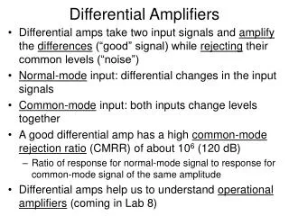
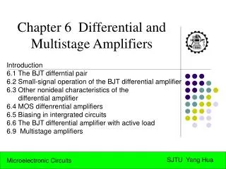
Differential and Multistage Amplifiers. 1. Figure 7.1 The basic MOS differential-pair configuration. Figure 7.2 The MOS differential pair with a common-mode input voltage v CM. Figure 7.3 Circuits for Exercise 7.1. Effects of varying v CM on the operation of the differential pair.

E N D
Differential and Multistage Amplifiers 1
Figure 7.1 The basic MOS differential-pair configuration. Microelectronic Circuits - Fifth Edition Sedra/Smith
Figure 7.2 The MOS differential pair with a common-mode input voltage vCM. Microelectronic Circuits - Fifth Edition Sedra/Smith
Figure 7.3 Circuits for Exercise 7.1. Effects of varying vCM on the operation of the differential pair. Microelectronic Circuits - Fifth Edition Sedra/Smith
Figure 7.3(Continued) Microelectronic Circuits - Fifth Edition Sedra/Smith
Figure 7.4 The MOS differential pair with a differential input signal vid applied. With vid positive: vGS1>vGS2, iD1>iD2, and vD1<vD2; thus (vD2-vD1) will be positive. With vid negative: vGS1<vGS2, iD1<iD2, and vD1>vD2; thus (vD2-vD1) will be negative. Microelectronic Circuits - Fifth Edition Sedra/Smith
Figure 7.5 The MOSFET differential pair for the purpose of deriving the transfer characteristics, iD1 and iD2 versus vid=vG1 – vG2. Microelectronic Circuits - Fifth Edition Sedra/Smith
Figure 7.6 Normalized plots of the currents in a MOSFET differential pair. Note that VOV is the overdrive voltage at which Q1 and Q2 operate when conducting drain currents equal to I/2. Microelectronic Circuits - Fifth Edition Sedra/Smith
Figure 7.7 The linear range of operation of the MOS differential pair can be extended by operating the transistor at a higher value of VOV. Microelectronic Circuits - Fifth Edition Sedra/Smith
Figure 7.8 Small-signal analysis of the MOS differential amplifier: (a) The circuit with a common-mode voltage applied to set the dc bias voltage at the gates and with vid applied in a complementary (or balanced) manner. (b) The circuit prepared for small-signal analysis. (c) An alternative way of looking at the small-signal operation of the circuit. Microelectronic Circuits - Fifth Edition Sedra/Smith
Figure 7.9(a) MOS differential amplifier with ro and RSS taken into account. (b) Equivalent circuit for determining the differential gain. Each of the two halves of the differential amplifier circuit is a common-source amplifier, known as its differential “half-circuit.” Microelectronic Circuits - Fifth Edition Sedra/Smith
Figure 7.10(a) The MOS differential amplifier with a common-mode input signal vicm. (b) Equivalent circuit for determining the common-mode gain (with ro ignored). Each half of the circuit is known as the “common-mode half-circuit.” Microelectronic Circuits - Fifth Edition Sedra/Smith
Figure 7.11 Analysis of the MOS differential amplifier to determine the common-mode gain resulting from a mismatch in the gm values of Q1 and Q2. Microelectronic Circuits - Fifth Edition Sedra/Smith
Figure 7.12 The basic BJT differential-pair configuration. Microelectronic Circuits - Fifth Edition Sedra/Smith
Figure 7.13 Different modes of operation of the BJT differential pair: (a) The differential pair with a common-mode input signal vCM. (b) The differential pair with a “large” differential input signal. Microelectronic Circuits - Fifth Edition Sedra/Smith
Figure 7.13 (Continued) (c) The differential pair with a large differential input signal of polarity opposite to that in (b). (d) The differential pair with a small differential input signal vi. Note that we have assumed the bias current source I to be ideal (i.e., it has an infinite output resistance) and thus I remains constant with the change in vCM. Microelectronic Circuits - Fifth Edition Sedra/Smith
Figure E7.7 Microelectronic Circuits - Fifth Edition Sedra/Smith
Figure 7.14 Transfer characteristics of the BJT differential pair of Fig. 7.12 assuming a. 1. Microelectronic Circuits - Fifth Edition Sedra/Smith
Figure 7.15 The transfer characteristics of the BJT differential pair (a) can be linearized (b) (i.e., the linear range of operation can be extended) by including resistances in the emitters. Microelectronic Circuits - Fifth Edition Sedra/Smith
Figure 7.16 The currents and voltages in the differential amplifier when a small differential input signal vid is applied. Microelectronic Circuits - Fifth Edition Sedra/Smith
Figure 7.17 A simple technique for determining the signal currents in a differential amplifier excited by a differential voltage signal vid; dc quantities are not shown. Microelectronic Circuits - Fifth Edition Sedra/Smith
Figure 7.18 A differential amplifier with emitter resistances. Only signal quantities are shown (in color). Microelectronic Circuits - Fifth Edition Sedra/Smith
Figure 7.19 Equivalence of the BJT differential amplifier in (a) to the two common-emitter amplifiers in (b). This equivalence applies only for differential input signals. Either of the two common-emitter amplifiers in (b) can be used to find the differential gain, differential input resistance, frequency response, and so on, of the differential amplifier. Microelectronic Circuits - Fifth Edition Sedra/Smith
Figure 7.20 The differential amplifier fed in a single-ended fashion. Microelectronic Circuits - Fifth Edition Sedra/Smith
Figure 7.21(a) The differential half-circuit and (b) its equivalent circuit model. Microelectronic Circuits - Fifth Edition Sedra/Smith
Figure 7.22(a) The differential amplifier fed by a common-mode voltage signal vicm. (b) Equivalent “half-circuits” for common-mode calculations. Microelectronic Circuits - Fifth Edition Sedra/Smith
Figure 7.23(a) Definition of the input common-mode resistance Ricm. (b) The equivalent common-mode half-circuit. Microelectronic Circuits - Fifth Edition Sedra/Smith
Figure 7.24 Circuit for Example 7.1. Microelectronic Circuits - Fifth Edition Sedra/Smith
Figure 7.25(a) The MOS differential pair with both inputs grounded. Owing to device and resistor mismatches, a finite dc output voltage VO results. (b) Application of a voltage equal to the input offset voltage VOS to the terminals with opposite polarity reduces VO to zero. Microelectronic Circuits - Fifth Edition Sedra/Smith
Figure 7.26(a) The BJT differential pair with both inputs grounded. Device mismatches result in a finite dc output VO. (b) Application of the input offset voltage VOS;VO/Ad to the input terminals with opposite polarity reduces VO to zero. Microelectronic Circuits - Fifth Edition Sedra/Smith
Figure 7.27 A simple but inefficient approach for differential to single-ended conversion. Microelectronic Circuits - Fifth Edition Sedra/Smith
Figure 7.28(a) The active-loaded MOS differential pair. (b) The circuit at equilibrium assuming perfect matching. (c) The circuit with a differential input signal applied, neglecting the ro of all transistors. Microelectronic Circuits - Fifth Edition Sedra/Smith
Figure 7.29 Determining the short-circuit transconductance Gm;io/vidof the active-loaded MOS differential pair. Microelectronic Circuits - Fifth Edition Sedra/Smith
Figure 7.30 Circuit for determining Ro. The circled numbers indicate the order of the analysis steps. Microelectronic Circuits - Fifth Edition Sedra/Smith
Figure 7.31 Analysis of the active-loaded MOS differential amplifier to determine its common-mode gain. Microelectronic Circuits - Fifth Edition Sedra/Smith
Figure 7.32 (a) Active-loaded bipolar differential pair. (b) Small-signal equivalent circuit for determining the transconductance Gm;io/vid. (c) Equivalent circuit for determining the output resistance Ro;vx/ix. Microelectronic Circuits - Fifth Edition Sedra/Smith
Figure 7.33 Analysis of the bipolar active-loaded differential amplifier to determine the common-mode gain. Microelectronic Circuits - Fifth Edition Sedra/Smith
Figure 7.34 The active-loaded BJT differential pair suffers from a systematic input offset voltage resulting from the error in the current-transfer ratio of the current mirror. Microelectronic Circuits - Fifth Edition Sedra/Smith
Figure 7.35 An active-loaded bipolar differential amplifier employing a folded cascode stage (Q3 and Q4) and a Wilson current mirror load (Q5, Q6, and Q7). Microelectronic Circuits - Fifth Edition Sedra/Smith
Figure 7.36 (a) A resistively loaded MOS differential pair with the transistor supplying the bias current explicitly shown. It is assumed that the total impedance between node S and ground, ZSS, consists of a resistance RSS in parallel with a capacitance CSS. (b) Differential half-circuit. (c) Common-mode half-circuit. Microelectronic Circuits - Fifth Edition Sedra/Smith
Figure 7.37 Variation of (a) common-mode gain, (b) differential gain, and (c) common-mode rejection ratio with frequency. Microelectronic Circuits - Fifth Edition Sedra/Smith
Figure 7.38 The second stage in a differential amplifier is relied on to suppress high-frequency noise injected by the power supply of the first stage, and therefore must maintain a high CMRR at higher frequencies. Microelectronic Circuits - Fifth Edition Sedra/Smith
Figure 7.39 (a) Frequency-response analysis of the active-loaded MOS differential amplifier. (b) The overall transconductance Gm as a function of frequency. Microelectronic Circuits - Fifth Edition Sedra/Smith
Figure 7.40 Two-stage CMOS op-amp configuration. Microelectronic Circuits - Fifth Edition Sedra/Smith
Figure 7.41 Equivalent circuit of the op amp in Fig. 7.40. Microelectronic Circuits - Fifth Edition Sedra/Smith
Figure 7.42 Bias circuit for the CMOS op amp. Microelectronic Circuits - Fifth Edition Sedra/Smith
Figure 7.43 A four-stage bipolar op amp. Microelectronic Circuits - Fifth Edition Sedra/Smith
Figure 7.44 Circuit for Example 7.4. Microelectronic Circuits - Fifth Edition Sedra/Smith
Figure 7.45 Equivalent circuit for calculating the gain of the input stage of the amplifier in Fig. 7.43. Microelectronic Circuits - Fifth Edition Sedra/Smith
Figure 7.46 Equivalent circuit for calculating the gain of the second stage of the amplifier in Fig. 7.43. Microelectronic Circuits - Fifth Edition Sedra/Smith