Download
1 / 48
480 likes | 485 Views
Lecture 4. Grid-based modelling. Outline introduction linking models to GIS basics of cartographic modelling modelling in GRID. Introduction. GIS provides: comprehensive set of tools for environmental data management limited spatial analysis functionality

E N D
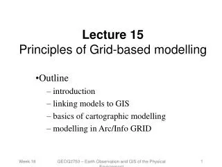
Lecture 4.Grid-based modelling Outline introduction linking models to GIS basics of cartographic modelling modelling in GRID GEOG5060 - GIS and Environment
Introduction • GIS provides: • comprehensive set of tools for environmental data management • limited spatial analysis functionality • but does provides framework of application • limited spatial analysis functionality may be addressed by linking models into GIS GEOG5060 - GIS and Environment
Spatial modelling issues • Model problems: • most models do not provide tools for data management and display, etc. • many models are aspatial • GIS provides: • framework of application • allows user to add spatial dimension (if not already built into the model) GEOG5060 - GIS and Environment
GIS-able models • Types of models applicable to integration with GIS include: • certain aspatial models • black box models • lumped models • all spatial models • distributed models • temporal models GEOG5060 - GIS and Environment
Linking models to GIS • Two basic methods of integrating models into the GIS framework: • soft or loose coupling • models and GIS are linked via file transfer • hard or tight coupling • models and GIS are linked directly through sharing common database • model programmed using GIS macros and functions GEOG5060 - GIS and Environment
Creating the link • How models are integrated into a GIS depends on: • the type model itself • the flexibility of the GIS as a modelling environment • the time and resources available • Fuzzy boundary between loose and tight coupling GEOG5060 - GIS and Environment
Loose coupling External data transfer MODEL G.I.S GIS database GEOG5060 - GIS and Environment
Tight coupling Internal data transfer MODEL GIS database G.I.S GEOG5060 - GIS and Environment
Example • GIS-based gas dispersion model • requirements: • an emergency planning decision support system is required for accident planning involving releases of chlorine gas from chemical plants • a dense gas dispersion model needs to be linked to a GIS to enable predictions of gas dispersion to be integrated with environmental data to assist in emergency planning procedures • loose or tight coupling? GEOG5060 - GIS and Environment
Questions… • Which model? • Which GIS? • Which data? • What level of coupling? GEOG5060 - GIS and Environment
Loose coupling approach • identify point of release (POR) and conditions of release (COR) • input POR and COR variables to model via keyboard input • run model • pass model results to GIS via file exchange • create model results data layer in GIS • integrate (overlay) with other data layers GEOG5060 - GIS and Environment
Tight coupling approach • identify POR and COR • run model • create POR and COR layers • model accesses GIS database directly for inputs at every increment of the model run to update basis for predictions • model creates new data layer in GIS database describing results • integrate (overlay) model results with other data layers GEOG5060 - GIS and Environment
Integrating GASTAR with Arc/Info GEOG5060 - GIS and Environment
Modelling testing • Testing models • verifying model output can present certain problems for the user • especially true if : • the model is complicated • two or more models are used • the data used is complex or of dubious accuracy or both! • long timescales are involved • the model is of the black box variety or if the user is unfamiliar with its workings GEOG5060 - GIS and Environment
Example • RUNMOD • a lumped catchment model of the hydrological cycle • lumped input: precipitation • lumped storage: soil store, groundwater store, channel store • lumped output: evapotranspiration, runoff • parameters governing infiltration, through flow, percolation, etc. can be altered to improve modelled outputs compared to measured outputs • this is a process known as calibration GEOG5060 - GIS and Environment
Questions… • What are the advantages of model calibration? • How could this particular model be integrated into a GIS framework? GEOG5060 - GIS and Environment
Modelling guidelines • In order to ensure that model results are as close to reality as possible the following guidelines apply: • ensure data quality • beware of making too many assumptions • match model complexity with process complexity • compare predicted results with empirical data where possible and adjust model parameters and constants to improve goodness of fit • use results with care! GEOG5060 - GIS and Environment
Basics of cartographic modelling • Mathematics applied to raster maps • often referred to as map algebra or ‘mapematics’ • e.g. combination of maps by: • addition • subtraction • multiplication • division, etc. • operations on single or multiple layers GEOG5060 - GIS and Environment
A definition “A generic means of expressing and organising the methods by which spatial variables and spatial operations are selected and used to develop a GIS model” GEOG5060 - GIS and Environment
5 7 4 A simple example… 4 1 3 2 3 6 Input 1 4 2 2 6 1 2 3 + 6 3 3 4 2 1 6 2 Input 2 4 6 4 3 1 3 2 4 = 7 7 6 6 13 5 7 7 Output 6 10 8 5 2 10 5 5 GEOG5060 - GIS and Environment
Question… • How determine topological relationships? i.e. Boolean: AND, NOT, OR, XOR • What is the arithmetic equivalent? GEOG5060 - GIS and Environment
Building spatial models • It is (in theory) surprisingly simple: • algebraic combination of: • OPERATORS and FUNCTIONS • rules and relationships • inputs (and outputs) • interfaces • run at the command line/menu interface • batch file • embedded in system macro/script • ‘hard’ programmed into system GEOG5060 - GIS and Environment
Problems in model building • knowledge • systems and processes • relationships and rules • compatability • input data available • outputs required • quality issues • data quality (accuracy, appropriateness, etc.) • model assumptions and generalisation • confidence and communication GEOG5060 - GIS and Environment
Modelling in Arc/Info GRID • Four basic categories of functions in map algebra: • local • focal • zonal • global • Operate on user specified input grid(s) to produce an output grid, the cell values in which are a function of a value or values in the input grid(s) GEOG5060 - GIS and Environment
Local functions • Output value of each cell is a function of the corresponding input value at each location • value NOT location determines result • e.g. arithmetic operations and reclassification • full list of local functions in GRID is enormous • Trigonometric, exponential and logarithmic • Reclassification and selection • Logical expressions in GRID • Operands and logical operators • Connectors • Statistical • Other local functions GEOG5060 - GIS and Environment
5 7 4 Local functions input 25 49 16 output = sqr(input) GEOG5060 - GIS and Environment
Some examples input output = reclass(input) output = log2(input) output = tan(input) GEOG5060 - GIS and Environment
Focal functions • Output value of each cell location is a function of the value of the input cells in the specified neighbourhood of each location • Type of neighbourhood function • various types of neighbourhood: • 3 x 3 cell or other • calculate mean, SD, sum, range, max, min, etc. GEOG5060 - GIS and Environment
5 7 4 Focal functions input 11 16 output = focalsum(input) GEOG5060 - GIS and Environment
Some examples input output = focalstd(input) output = focalvariety(input) output = focalmean(input, 20) GEOG5060 - GIS and Environment
Neighbourhood filters • Type of focal function • used for processing of remotely sensed image data • change value of target cell based on values of a set of neighbouring pixels within the filter • size, shape and characteristics of filter? • filtering of raster data • supervised using established classes • unsupervised based on values of other pixels within specified filter and using certain rules (diversity, frequency, average, minimum, maximum, etc.) GEOG5060 - GIS and Environment
1 2 1 3 4 1 1 2 3 1 2 4 5 1 2 2 1 2 4 1 1 2 4 5 2 Old class New class Supervised classification GEOG5060 - GIS and Environment
diversity 1 3 4 modal 2 4 5 1 2 4 minimum maximum mean Unsupervised classification 5 4 1 5 3 GEOG5060 - GIS and Environment
Zonal functions • Output value at each location depends on the values of all the input cells in an input value grid that shares the same input value zone • Type of complex neighbourhood function • use complex neighbourhoods or zones • calculate mean, SD, sum, range, max, min, etc. GEOG5060 - GIS and Environment
5 7 4 Zonal functions input Zone 2 zone Zone 1 9 7 7 7 9 7 7 7 9 9 9 7 output = zonalsum(zone, input) 9 9 9 7 GEOG5060 - GIS and Environment
Some examples input Input_zone 535.54 127 6280 766.62 160 10800 output = zonalthickness(input_zone) output = zonalmax(input_zone, input) output = zonalperimeter(input_zone) GEOG5060 - GIS and Environment
Global functions • Output value of each location is potentially a function of all the cells in the input grid • e.g. distance functions, surfaces, interpolation, etc. • Again, full list of global functions in GRID is enormous • euclidean distance functions • weighted distance functions • surface functions • hydrologic and groundwater functions • multivariate. GEOG5060 - GIS and Environment
5 7 4 Global functions input 6 7 8 9 5 6 7 8 4 5 6 7 output = trend(input) 4 5 6 6 GEOG5060 - GIS and Environment
Distance functions • Simple distance functions • calculate the linear distance of a cell from a target cell(s) such as point, line or area • use different distance decay functions • linear • non-linear (curvilinear, stepped, exponential, root, etc.) • use target weighted functions • use cost surfaces GEOG5060 - GIS and Environment
Some examples input source output = eucdistance(source) output = eucdirection(source) output = costdistance(source, input) GEOG5060 - GIS and Environment
COSTPATH example GEOG5060 - GIS and Environment
Conclusions • Linking/building models to GIS • Idea of maths with maps • surprisingly simple, flexible and powerful technique • basis of all raster GIS • Fundamental to spatial interpolation, distance and neighbourhood functions GEOG5060 - GIS and Environment
Workshop • Constructing models in Arc/Info GRID • Demonstration of GRID functions • Focal functions • Local functions • Global functions • Zonal functions • AML for GRID GEOG5060 - GIS and Environment
Practical • Facilities location using Arc/Info GRID • Task: Locate suitable sites for a wind farm in the Yorkshire Wolds • Data: The following datasets are provided… • Digital elevation model (50m resolution 1:50,000 OS Panorama data) • Contour data (10m interval 1:50,000 OS Panorama data) • ITE land cover map (25m resolution) • Roads (1:250,000 Meridian data) • Wind speed data GEOG5060 - GIS and Environment
Practical • Steps: • Formulate a location model based on available data and requirements for a wind farm • Pre-process data to create model input layers as required • Run model • Identify best location(s) GEOG5060 - GIS and Environment
Siting wind turbines GEOG5060 - GIS and Environment
Practical • Experience at simple cartographic model building • Experience with spatial modelling functions within Arc/Info GRID • Familiarity with locational models and wind farm siting in particular GEOG5060 - GIS and Environment
Next week… • Terrain modelling 1: the basics • DEMs and DTMs • Derived variables • Example applications • Workshop: Terrain modelling in Arc/Info and Grid • Practical:Using DEMs GEOG5060 - GIS and Environment