Download
1 / 77
790 likes | 1.19k Views
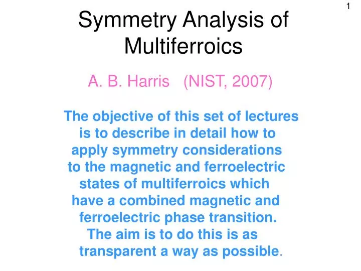
1. Symmetry Analysis of Multiferroics. The objective of this set of lectures is to describe in detail how to apply symmetry considerations to the magnetic and ferroelectric states of multiferroics which have a combined magnetic and ferroelectric phase transition.

E N D
1 Symmetry Analysis of Multiferroics The objective of this set of lectures is to describe in detail how to apply symmetry considerations to the magnetic and ferroelectric states of multiferroics which have a combined magnetic and ferroelectric phase transition. The aim is to do this is as transparent a way as possible. A. B. Harris (NIST, 2007)
2 OUTLINE • Setting the Stage • Symmetry of the Quadratic Free Energy A. Physics of this Free Energy B. Eigenvector Condition (TbMnO3) C. Group of the Wavevector (TbMn2O5 , YMn2O5) D. Impose Inversion Symmetry E. Introduce and Analyze Order Parameters • Consider Quartic Terms in the Free Energy • Construct the Magnetoelectric Coupling using the Symmetry of the Order Parameters V. Discussion
3 HISTORICAL REMARKS Prior to our 2005 Physical Review Letter1 it was not recognized that, in addition to the symmetry operations which leave the wave- ector invariant, one could exploit inversion symmetry. (This may have been recognized in some quarters, but certainly none of the multiferroic community knew it!) This is docu- mented in Ref. 2, on which these notes are based and to which citation may be made. A reader who understands representation theory can skip to slide #27!!
4 INVERSE SUSCEPTIBILITY The susceptibility is a key quantity in continuous transitions like those we are about to study. One is used to saying that the susceptibility diverges at a continuous transition. Alternatively, one can plot the free energy, F, (see the appendix) of a ferromagnet versus the magnetization, M. By time reversal only even powers of M can appear. The actual value of M is the one which minimizes F. Free energy F = (T-Tc)M2 + uM4 for a sequence of temperatures T< < Tc < T1 < T2. Note that the free energy is unstable relative to the formation of long-range order for T < Tc
5 INVERSE SUSCEPTIBILITY Ferromagnet For small H the magnetization M is T2 > T1 > Tc The coefficient of M2 is the inverse susceptibility: In the Appendix we allow for all Fourier components: For a ferromagnet the instability first occurs at q=0 as one reduces the temperature. When the first Fourier component condenses, the others are inhibited from condensing because there is a finite amount of spin to go around.
6 INVERSE SUSCEPTIBILITY For the antiferromagnet the instability leads to up-down-up-down spins, i. e. aq = p. Observe that if you have a plot of the susceptibility versus wavevector, you don’t have to know whether the system is ferromagnetic or anti- ferromagnetic: the location of the minimum in inverse chi tells you which it is. Antiferromagnet The instability occurs at wave- vector q=p/a
7 WAVEVECTOR SELECTION:INCOMMENSURATE SPINS For competing interactions, the minimum in inverse chi can be anywhere in the zone, as at right. Incommensurate Magnet The minimum in inverse chi locates the wavevector of the ordered state. This is often referred to as “wavevector selection.” So far we have treated M as a scalar, as it is for the Ising model. What happens if M is a vector? T = Tc T = T1 > Tc T = T2 > T1
8 INVERSE SUSCEPTIBILITY Suppose we have vector spins with an easy axis along z. Then Where K>0 is the anisotropy energy. Here as T approaches Tc from above, only Mz becomes unstable relative to long-range order. As another example suppose the free energy is (Continued next slide)
9 INVERSE SUSCEPTIBILITY How do we deal with Now we have an anisotropy tensor, which we can diagonalize to find the anisotropies associated with each principal axis. Keeping only the order para- meter associated with the easiest axis, , we have This example teaches us that if the free energy is a quadratic form, ordering takes place in the channel defined by the eigenvector associated with the eigenvalue that is vanishing.
10 INCOMMENSURATE CHI Now we consider the free energy of a system which has n>1 vector spins in the unit cell: Let Sa(R,t) denote the a-component of the spin at position t within the unit cell at R. Then where sa(q,t) is complex with sa(-q,t)=sa(q,t)*. The quadratic free energy is the Hermitian form This quadratic form has complex-valued eigen- vectors which we can normalize, but they have an arbitrary phase factor (which I will discuss later). Obviously we focus on the critical eigen- value, i. e. the one that first becomes unstable.
11 INTERPRETATION For each value of the wavevector we have 3n eigen- ectors and 3n eigenvalues. As the temperature is lowered we have wavevector selection: at some q, one of these eigenvalues will become unstable. This determines the wavevector of the ordered state (at least for temperature just below Tc). Now consider the eigenvector. Its normalization is not fixed by the quadratic free energy. The quartic terms fix the nor- malization and give the square root temperature dependence characteristic of mean field theory. Reminder: all the coefficients of the critical eigen- vector (which represents the Fourier transform of the spin distribution) are complex-valued. Note: we reject the possibility of accidental degeneracy. Degeneracy can only occur if symmetry requires it.
12 INTERPRETATION So we write the eigenvector Y as where the components inside the square bracket are normalized so that the sum of the squares of their magnitudes is unity. I will discuss the phase f later. The amplitude X varies as (Tc-T)1/2. sa,t is the complex amplitude of the wave of the a-component of the t sublattice. So the eigenvector tells us the pattern into which the spins order, as we will see in a moment.
13 APPLICATION One might attempt to write down and anlyze the matrix of coefficients F. That is a hopeless task because our microscopic models are not reliable. Instead, we use the symmetry of the crystal to limit the possible eigen- vectors which are determined by fitting the diffraction data. The standard approach is to invoke group theory. I will avoid that as much as possible. Instead I will invoke the principle that first-year graduate students learn: if a set G1, G2, …of mutually commuting opera-tors commute with the Hamiltonian, then the eigen-vectors of the Hamiltonian can be classified according to their eigenvalues g1, g2, … In the language of group theory, this case is the case when all the irreducible representations are one dimensional.
14 CALCULATION The essential input we require is the symmetry of the incommensurate wavevector (usually as determined by neutron diffraction) i. e. the symmetry operations of the crystal which also leave this wavevector invariant. Since we are concerned with phase transitions in which ferroelectricity appears in coincidence with magnetic ordering, spatial inversion I is a significant symmetry operation, although it does not usually leave the wavevector invariant. So I’m afraid we have to actually confront the crystal structure of the paramagnetic phase.
15 = Mn = Tb EXAMPLE A: TbMnO3 The space group opera- tions3 are defined in Table I and the ion positions are listed in Table II (x=0.9836, y=0.0810)4. The figure below shows the mirror plane (z=1/4) for mz and the glide plane (x=3/4) for mx with associated translation uy = b/2. From neutron diffraction5,6 the wavevector lies along b (i. e. y) and in rlu is q= 0.28. The wavevector is invariant under mx and mz. Table I: General positions for Pbnm (TMO).3,4 Here x means –x. Table II: Mn and Tb positions.4
16 Eigenfunctions for TbMnO3 (TMO) • In Table III I give the eigenfunctions for TMO. First I explain how to read this table. In each column headed by the symmetry label (Gn) I list the components of eigenfunctions on the sites 1 – 8 as labeled in Table II. The three numbers in each box are for • the x, y, and z components. These eigenfunctions are eigenfunctions of mx and mz with respective eigenvalues l(mx) and l(mz). Here • = exp(ipq), where q is the incommensurate wavevector in reciprocal lattice units (rlu), so in ``real” units, it is 2pq/b. Table III: Eigen- vectors. L = exp(ipq).
17 EIGENFUNCTIONS The eigenfunction for G1 has five parameters xM, yM, zM, zT1, and zT2 indicating that there are five independent eigenfunctions of this symmetry. So far, there is no restriction on these five complex parameters. As we will see below, inversion symmetry places important constraints on these parameters. On the next slides we will show how the eigenvectors are easily constructed. Table III (repeated)
18 EIGENFUNCTIONS To construct eigenfunctions of mx and mz it is convenient to write Y in terms of subvectors as where each symbol is a vector with four components. X(M) has the x-components of the four Mn sublattices, Y(M) and Z(M) the y and z components, respectively, of the four Mn sublattices. Similarly, X(T), Y(T) , and Z(M) have the x, y, and z components, respectively, of the four Tb sublattices. The representation of Eq. (2) is convenient because the symmetry operations only interrelate the four components within a given symbol. Consequently, each eigenfunction has components only with in a single four-component subvector.
19 EIGENFUNCTIONS The main ideas involved in determining how spin functions transform are: 1) The transformed spin at r is obtained by OS acting on the spin which was at the original location [OR]-1 r, 2) exp(iqr) is a number and O does not act on it, and 3) the subscripts ``i” and ``f” mean ``before” and ``after” transformation. In Table IV we list the initial and final sites under the operations we will invoke. Table IV (at right): initial site, ti, sites, tf, after mx, mz, and I. The sites are numbered according to Table II.
20 EIGENFUNCTIONS To construct the eigenfunctions of mx and mz, we need to discuss how the symmetry opera- tions act on Fourier transforms of spin functions like sx(q,1). First of all, spin is a pseudovector, so the mirror ma does’t reverse the sign of the a-component of spin but does reverse the sign of the other components.Let O denote an operator acting on spin and space, OR (OS) an operator acting only on space (spin), and lower case denote a Fourier transform. On the next slide we indicate the effect of a symmetry operator O=OR OS on a Fourier transform.
21 EIGENFUNCTIONS OR = a point group operation GO + a translation uO: so that (since GO leaves q invariant) Thus, the final result is
22 EIGENFUNCTIONS The result of the previous slide was For mz, u0=0, and for mx, q.u0=pq (recall rlu!). Also, OS gives a plus or minus sign. Thus where the sign depends on O and a and t (t’) is the initial (final) sublattice. Thus for the pseudovector spins, with L = exp(ipq), where xab = -1, except that xaa = +1, so that mz2 = 1 and mx2 = L2 . Note: ( t’)’=t.
23 EIGENFUNCTIONS Now we show how the eigenvectors are constructed. For instance, to construct the eigenvector scaled by xM, we assign m1x the value 1 and then deduce the other components according to the symmetry (l ‘s). So we introduce projection operators To check the effect of Px, use mx2 = L2 = l(mx)2:
24 EIGENFUNCTIONS Thus P PxPz projects an eigenfunction of both mx and mz with respective eigenvalues l(mx) and l(mz). We extend the notation of Eq. (2) so that (a,b,c,d)sT represents a subvector S(T), whose four components are a, b, c, and d, and where s=x, y, or z (to label components) and T=M or T (for Mn or Tb). We now illustrate the use of these projection opera- tors to construct eigenfunctions of mx and mz. To get the eigenfunction Y scaled by xM , we let the projection operator act on X(M) = [1,0,0,0]xM in the notation of Eq. (2):
25 EIGENFUNCTIONS In the first line we used Table IV which tells us that mz takes site #1 into site #3 and Eq. (5) with xzx=-1. In the third line Table IV tells us that mx takes site #1 into site #2 and #3 into #4 and we used Eq. (4) with xxx=1. The above eigenvector regulates the x-components on the Mn sites. To get the amplitudes for G1 set l(mz)=1 and l(mx)=L. This leads to Y=[1,1,-1,-1]xM in agree- ment with the eigenvector of Table IV scaled by xM.
26 EIGENFUNCTIONS To further illustrate the construction of the eigen- vectors we apply the projection operator to the Tb wavefunction [1,0,0,0]xT : So for l(mz)=+1, there are no eigenvectors of the x-component. Otherwise the eigenfunction covers only sites #5 and #8. One can verify that the above result agrees with Table III. Enough checks!
27 EIGENFUNCTIONS: SUMMARY For convenience I repeat Table III at right. For those rejoining here, each column contains the most general eigenvector having the symmetry specified either by the eigenvalues of the symmetry operators, or by the irreducible representation G. At this stage of the development the 5 (or 7) free parameters may assume arbitrary complex values. The guiding principle is that we do not admit the possibility of accidental degeneracy. When ordering takes place only one symmetry eigen-vector can condense. The Fourier transform of the spin distribution is proportional to this ``critical” eigen-vector. The symmetry (G) and the amplitudes (x, y, z) are determined to best fit to diffraction data.
28 INVERSION SYMMETRY Up to now our results are absolutely standard. It is often said (in reviews7) that the only symmetries that can be exploited are those that leave the wavevector invariant. This is not so because when one has inversion symmetry, the free energy clearly must be invariant with respect to inversion.1,2,8 We now analyze the consequences of that. We assume that only a single representation is critical and write the free energy as an Hermitian form in in the amplitudes (which we here denote Qi) of one of the columns (G) of Table III: So Q1(G) = xM, Q2(G) = yM, etc.
29 INVERSION Clearly, we now have to determine how inversion I transforms the coordinates Q. For that purpose we modify the derivation of Eq. (3) so that it applies to I. Replace ``leaves q invariant” by ``changes the sign of q.” Thereby we get What does this mean? The initial and final sites are given in Table IV. For the Mn sites, they are at centers of symmetry so tf = ti. So Isa(q,n)=sa(q,n)* for Mn sites (n=1,2,3,4). For the Tb sites the pairs of initial and final sites are 5 and 7 and 6 and 8, so Isa(q,5)=sa(q,7)* and Isa(q,6)=sa(q,8)*.
30 INVERSION Now we deduce the effect of inversion on the sym- metry adapted coordinates, denoted Qn(G), which are the amplitudes in terms of the eigenfunctions of Table III. As an illustration we consider the coordinates of G1 from column 1 of Table III:
31 INVERSION From the discussion of Eq. (6) one sees that Now write the free energy (for G = G1) in terms of the Q’s and require invariance under inversion: Here and below we invoke the convention that Roman letters are real and Greek ones complex. Thus
32 INVERSION To repeat: We now need to study how inversion affects the matrix. For example, IQ1* Q4 = Q5* Q1. After inversion the 5,1 element of the matrix is the old 1,4 element. A simpler example: IQ1* Q2 = Q2* Q1, so after inversion the 2,1 element is the old 1,2 element.
33 INVERSION Since these two forms have to be equal no matter how we choose the Q’s, the matrices have to be equal. Thus a, b, and e must be real and Thus the free energy is of the form (with Roman letters real and Greek ones complex). The critical eigenvector is an eigenvector of the above matrix.
34 INVERSION To repeat: we found the free energy to be Because of the special form of this matrix (due to invoking inversion symmetry) the eigenvector is shown in the Appendix to be of the form6 where the subscript Q says that the components are Q1, Q2, Q3, … and we normalize by a2+b2+c2+2|r|2=1. Since the eigenvalue problem takes place in a complex vector space, we can not omit the arbitrary phase f. We discuss this result below.
35 INVERSION We now discuss the result of the last slide: Previously (in Table III) we showed that symmetry led to an eigenvector of symmetry G1 which had five complex coefficients. Now we see that apart from an overall phase factor, three of these are real, and the other two (for Tb), rather than being independent complex numbers are the complex conjugates of one another: So instead of having 5 complex amplitudes to fit the diffraction data, we have three real and one complex parameter. The result for G = G3 is similar. The result for G2 (G4) is (see the Appendix)
36 INVERSION So at right we have updated Table III to take account of inversion symmetry. The eigen- functions of each symmetry Gn should be assigned an inde- pendent phase factor fn and amplitude An. If only one symmetry is present, the phase is usually irrelevant. But if two symmetries are simultaneously present, the phases matter because the relative phase has significance, as we shall see. Reminder: Roman letters are real and Greek ones complex. As Table III, but with Inversion symmetry.
37 ORDER PARAMETERS We now discuss how the magnetic structure can be described by order parameters.2,8 Suppose that the structure has Gn symmetry and the spin wavefunction is put into the form of Eq. (8). How do we think about an order parameter? Here the order parameter has to be complex because any phase is allowed in Eq. (8). As a function of temperature the normalized eigen- vector will be essentially constant, and only the magnitude A will vary. So we identify the complex order parameter as where An is real.
38 ORDER PARAMETERS The order parameter inherits the symmetry of the representation Gn. Thus At right is the phase diagram9 of TMO. As one cools at H=0 throughT> = 40K, order in s3 appears6 in the HTI (high-temperature incommensurate) phase.8 Then at T=28K additional order in s2 appears6 in the low temperature (LTI) phase. Cooling at H>10T leads to a different phase. The polarization is nonzero only in the LTI phases. TMO Para P=0
39 MAGNETIC STRUCTURE Here I discuss qualitatively the magnetic structure. Neutron diffraction6 indicates that in the HTI phase the ordering with s3 (i. e. G3) involves the spins pointing along the b (i. e. y) axis. Since the a, b, and c directions are inequivalent, one axis must be easiest, and obviously this is the b axis. Note that the pattern of sublattice spins is (++--). The quartic terms in the free energy favor fixed spin length8 which is not consistent with a collinear sinusoidal state. Thus, it is not surprising8,10 that a phase transition occurs at lower temperature where transverse order appears along the c axis scaled by the order parameter s2, for G2. The pattern of these transverse moments is again (++--) indicating nearly isotropic interactions.
40 PHENOMENOLOGY This behavior is consistent with the following simple phenomenological Landau expansion: and is consistent with the famous review of incommensurate systems by Nagamiya.10 It is not obvious that the above free energy ensures that the wavevectors of the two order parameters are equal. If the interactions are nearly isotropic, one would expect this to be the case. Within Landau theory the term that locks to two order parameters is of the form8 where u<0 and this term only exists if q2 = q3.
41 MAGNETOELECTRIC COUPLING Now we discuss the Landau theory of magneto- electric (ME) coupling V.1,2,8 Order B is induced by order A if there is a term in the free energy linear in B times 2 (or more) powers of A. Time reversal invariance ensures that such a term linear in the magnetization can not occur, so the polarization P can not induce magnetic order. But magnetization can induce P. The interaction we seek is therefore of the form V = ss P and the ME free energy is then where the electric susceptibility cE is finite since we assume that without magnetism there is little tendency to have a spontaneous polarization.
42 ME COUPLING The ME coupling is schematically of the form Where c is a constant. Now minimize with respect to Pa: so this interaction does just what we want: it induces a polarization only when ss is nonzero.
43 ME COUPLING As we argued, the magnetoelectric interaction V is linear in P and quadratic in the magnetic order parameters. To conserve wavevector V is where G is a reciprocal lattice vector and delta is unity if q+q’=G and is zero otherwise. We drop the Umklapp term with G nonzero (for which see Ref. 11). Then we have
44 ME COUPLING Warning: the discussion that follows applies to TMO. For different symmetry systems the ME Interaction need not assume the form found be- low.2,12 In TMO, V must be invariant with respect to mx, mz, and I. To handle the cases that will be of interest to us, let us assume that there are two irreducible representations (irreps) present. Gr and Gs. In Eq. (10) the term with n=m is zero because it changes sign under I. Physically this reflects the fact that a single wave has a center of symmetry which, for an incommensurate q, can be as close to an inversion center of the lattice as you like. Thus
45 ME COUPLING To repeat: This has to be invariant under mz. Using Eq. (9) we have This equalsV only if mzPa=-Pa, i. e. for a=z (i. e. c). So One can show, using Eq. (9) that V is invariant under mx.
46 ME COUPLING We have V as This has to be invariant under inversion. We have To have IV = V, az must be imaginary: az=ir, with r real. We set sn(q) = |sn| exp (ifn). Then The polarization in TMO (at low H) is only found8 in the LTI phase where it lies along c (i. e. z) as in (11).
47 ME COUPLING The appearance of the relative phase is easily understood. The phase of the irrep regulates the location of origin of the cosine wave. The wave has inversion symmetry about this point. So, if the two irreps have their origin at the same point, i. e. if f2 = f3, then the entire structure has inversion symmetry about a lattice site. The fact that P is proportional to |s2 s3| also agrees with experiment8 in that the temperature depend- ence of Pz looks like that of an order parameter and not (order parameter)2. This happens because the HTI order parameter s3 is more or less saturated by the time one gets into the LTI phase.
48 HIGH FIELD PHASE In the high field phase (see the figure on slide #38) the polarization lies alog a (i. e. x) in the analog of the LTI phase. Thus the magnetic structure must be s3 + sn such that their product transforms like Pa. For the product to be odd under mx, we need n=1 or 4. For it to be even under mz, we need n=1 or 3. So this analysis indicates that n=3. (This was first predicted in Ref. 13.) It should be noted that having a different irrep does not necessarily mean a totally unrelated structure. It may simply mean that the structure has been rotated. Because different spin components transform different under symmetry operations, this causes a change in the irrep.
49 TbMn2O5 (T25) T25’s space group is Pbam,14,15 whose symmetry operations are in Table VI and whose ion positions are in Table VII. Table VI. Pbam space group operations.3 Below T=43K, T25 has a commen- surate phase with q=(1/2,0,1/4) and an incommensurate phase with q=(0.48, 0, 0.32).16 Since the irreps for T25 are two dimensional, the simple method used above is clumsy.2 An alternate way, used here, is to supplement the standard analysis by including inversion symmetry. Table VII. Positions of spins in T25: x=0.09, y=-0.15, z=0.25,14 X=0.14 and Y=0.17.15
50 T25 The standard analysis (without inversion symmetry) for the wavevector (0.50, 0, qz) leads to Table VIII, which is read just as Table III, except that the two columns do not represent dif- ferent symmetry irreps, but rather transform like two columns of the same irrep. Since the two columns are degenerate in free energy, the actual spin function is a linear combination (determined by a fit to diffraction data) of the two columns. The complex coefficients s1 and s2 are the order parameters. Table VIII for T25.