Download
1 / 48
480 likes | 601 Views
Morphology and Spatial Distribution of Cinder Cones at Newberry Volcano, Oregon: Implications for Relative Ages and Structural Control on Eruptive Process. Steve Taylor Earth and Physical Sciences Department Western Oregon University Monmouth, Oregon 97361. Introduction Geologic Setting

E N D
Morphology and Spatial Distribution of Cinder Cones at Newberry Volcano, Oregon: Implications for Relative Ages and Structural Control on Eruptive Process Steve Taylor Earth and Physical Sciences Department Western Oregon University Monmouth, Oregon 97361
Introduction • Geologic Setting • Morphometric Analysis • Cone Alignment Analysis • Summary and Conclusion
History of Newberry Work at Western Oregon University 2000 Friends of the Pleistocene Field Trip to Newberry Volcano 2002-2003 Giles and others, GIS Compilation and Digitization of Newberry Geologic Map (after MacLeod and others, 1995) 2003 Taylor and others, Cinder Cone Volume and Morphometric Analysis I (GSA Fall Meeting) 2005 Taylor and others, Spatial Analysis of Cinder Cone Distribution II (GSA Fall Meeting) 2007 Taylor and others, Synthesis of Cinder Cone Morphometric and Spatial Analyses (GSA Cordilleran Section Meeting) 2001-Present Templeton, Petrology and Volcanology of Pleistocene Ash-Flow Tuffs (GSA Cordilleran Meeting 2004; Oregon Academy of Science, 2007; GSA Annual Meeting 2009; AGU Annual Meeting 2010) 2011-Present Taylor and WOU Students, ES407 Senior Seminar Project, Pilot Testing of Lidar Methodologies on Cinder Cone Morphometry NOTE: Work presented today was conducted in pre-Lidar days mid-2000’s
Geology after Walker and MacLeod (1991); Isochrons in 1 m.y. increments (after MacLeod and others, 1976)
Basaltic Flows (Pl.- H) Tepee Draw Tuff Caldera Cinder Cones “Qc”
Cinder Cone Morphology and Degradation Over Time Wcr Wcr = crater diameter Wco = cone basal diameter Hco = cone height S = average cone slope Hco S (Dohrenwend et al., 1986) Wco MASS WASTING AND SLOPE WASH PROCESSES: Transfer primary cone mass to debris apron • Cone Relief Decreases • Cone Slope Decreases • Hco/Wco Ratio Decreases • Loss of Cater Definition • Increased Drainage Density Time (Valentine et al., 2006)
Cone AlignmentVia Fracture-Related Plumbing Newberry: Junction of Tumalo-Brothers-Walker Rim Fault Zones Rooney et al., 2011
Cinder Cone Research Questions Are there morphologic groupings of ~400 cinder cones at Newberry? Can they be quantitatively documented? Are morphologic groupings associated with age and state of erosional degradation? Are there spatial patterns associated with the frequency, occurrence, and volume of cinder cones? Are there spatial alignment patterns? Can they be statistically documented? Do regional stress fields and fracture mechanics control the emplacement of cinder cones at Newberry volcano?
Methodology • Digital Geologic Map Compilation / GIS of Newberry Volcano (after McLeod and others, 1995) • GIS analysis of USGS 10-m DEMs • Phase 1 Single Cones/Vents (n = 182) • Phase 2 Composite Cones/Vents (n = 165) • Morphometric analyses • Cone Relief, Slope, Height/Width Ratio • Morphometric Classification • Volumetric Analyses • Cone Volume Modeling • Volume Distribution Analysis • Cone Alignment Analysis • Two-point Line Azimuth Distribution • Comparative Monte Carlo Modeling (Random vs. Actual)
Single Cone DEM Example Composite ConeDEM Example (n = 182) COMPOSITE (n = 165)
Reject Ho Reject Ho Reject Ho Single Cones
“Youthful” “Mature” Northern DomainGroup I: n = 26 (14%) Group II: n = 76 (42%) Southern DomainGroup I: n = 16 (9%)Group II: n = 64 (35%) Single Cones
VOLUME METHODOLOGYClip cone footprint from 10-m USGS DEM (Rectangle 2x Cone Dimension)Zero-mask cone elevations, based on mapped extent from MacLeod and others (1995)Re-interpolate “beheaded” cone elevations using kriging algorithmCone Volume = (Cone Surface – Mask Surface) Original DEM ofLava Butte Masked DEM ofLava Butte
CONE VOLUME SUMMARY(SINGLE AND COMPOSITE) Cubic Meters
Cone lineaments anyone? Question: How many lines can be created by connecting the dots between 296 select cone center points?
Answer: Total Lines = [n(n-1)]/2 = [296*295]/2 = 43,660 possible line combinations Follow-up Question: Which cone lineaments are due to random chance and which are statistically and geologically significant?
METHODS OF CONE LINEAMENT ANALYSIS Frequency Azimuth “POINT-DENSITYMETHOD”(Zhang andLutz, 1989) GIS Frequency “TWO-POINTMETHOD”(Lutz, 1986) Azimuth
CONE TWO-POINT ALIGNMENT ANALYSIS (after Lutz, 1986) NULL HYPOTHESISDistribution of Actual Cone Alignments = Random Cone Alignments EXPECTED ALIGNMENT FREQUENCY:FEXP = (n*(n-1) / (2*k)) n = No. of Cinder Cones k = No. of Azimuthal Bins NORMALIZED ALIGNMENT FREQUENCY:FNORM = (FEXP / FAVG) * FOBS FNORM = normalized bin frequency FEXP = expected bin frequency FAVG = average random bin frequency FOBS = observed bin frequency CRITICAL VALUE:LI = [(FEXP / FAVG) * FAVG] + (tCRIT * RSTD) FEXP = expected bin frequency FAVG = average random bin frequency RSTD = stdev of random bin frequency tCRIT = t distribution (a = 0.05) Normalized Two-Point Cone Azimuths 95% Critical Value Random Two-Point Cone Azimuths n = 296 / replicateReplicates = 300 Actual Two-Point Cone Azimuths n = 296Line Segments = 43,660
TWO-POINT ANALYSIS RESULTS NORTH DOMAIN SOUTH DOMAIN 95% Critical Value 95% Critical Value n = 149 / replicateReplicates = 300 n = 147 / replicateReplicates = 300 n = 149 conesLine Segments = 11,026 n = 147 conesLine Segments = 10,731
POINT-DENSITY METHOD(Zhang and Lutz, 1989) 1-km wide filter strips with 50% overlapFilter strip-sets rotated at 5-degree azimuth incrementsTally total number of cones / strip / azimuth binCalculate cone density per unit areaCompare actual densities to random (replicates = 50)Normalize Cone Densities: D = (d – M) / S D = normalized cone density d = actual cone density (no. / sq. km) M = average density of random points (n = 50 reps) S = random standard deviationSignificant cone lineaments = >2-3 STDEV above random
I. CONE MORPHOLOGY • Degradation Models Through Time (Dohrenwend and others, 1986) • Diffusive mass wasting processes • Mass transfer: primary cone slope to debris apron • Reduction of cone height and slope • Loss of crater definition • Newberry Results (Taylor and others, 2003) • Group I Cones: Avg. Slope = 19-20o; Avg. Relief = 125 m; Avg. Hc/Wc = 0.19 • Group II Cones: Avg. Slope = 11-15o; Avg. Relief = 65 m; Avg. Hc/Wc = 0.14 • Group I = “Youthful”; more abundant in northern domain • Group II = “Mature”; common in northern and southern domains • Possible controlling factors include: degradation processes, age differences, climate, post-eruption cone burial, lava composition, and episodic (polygenetic) eruption cycles • II. CONE VOLUME RESULTS • Newberry cone-volume maxima align NW-SE with the Tumalo fault zone; implies structure has an important control on eruptive process
III. CONE ALIGNMENT PATTERNS • Newberry cones align with Brothers and Tumalo fault zones • Poor alignment correlation with Walker Rim fault zone • Other significant cone alignment azimuths: 10-35o, 80o, and 280-295o • Results suggest additional control by unmapped structural conditions • Cone-alignment and volume-distribution studies suggest that the Tumalo Fault Zone is a dominant structural control on magma emplacement at Newberry Volcano • IV. CONCLUDING STATEMENTS • This study provides a preliminary framework to guide future geomorphic and geochemical analyses of Newberry cinder cones • This study provides a preliminary framework from which to pose additional questions regarding the complex interaction between stress regime, volcanism, and faulting in central Oregon
ACKNOWLEDGMENTS Funding Sources: Western Oregon University Faculty Development Fund Cascades Volcano Association WOU Research Assistants and ES407 Senior Seminar Students: Jeff Budnick, Chandra Drury, Jamie Fisher, Tony Faletti Denise Giles, Diane Hale, Diane Horvath, Katie Noll, Rachel Pirot, Summer Runyan, Ryan Adams, Sandy Biester, Jody Becker, Kelsii Dana, Bill Vreeland, Dan Dzieken, Rick Fletcher
Extent of Hypothesized Newberry Ice Cap (Donnelly-Nolan and Jensen, 2009)
Cinder Cone Distribution Relative to Hypothesized Extent of Newberry Ice Cap Ice cap limit Single cones within ice limit Composite cones within ice limit Single cones outside ice limit Composite cones inside ice limit Caldera lakes
Cone Morphology Comparison Relative to Hypothesized Extent of Newberry Ice Cap Avg. Cone Long Axis/Short Axis Ratio No Significant Difference 1.35 1.30