Download
1 / 55
550 likes | 568 Views
Section 9.3 Tests About a Population Mean & Type I and II Errors. Section 9.3 Tests About a Population Mean. After this section, you should be able to… CONDUCT a one-sample t test about a population mean.

E N D
Section 9.3 Tests About a Population Mean & Type I and II Errors
Section 9.3Tests About a Population Mean After this section, you should be able to… • CONDUCT a one-sample t test about a population mean. • CONSTRUCT a confidence interval to draw a conclusion for a two-sided test about a population mean. • INTERPRET a Type I error and a Type II error in context, and give the consequences of each. • DESCRIBE the relationship between the significance level of a test, P(Type II error), and power.
Introduction Confidence intervals and significance tests for a population proportion p are based on z-values from the standard Normal distribution. Reminder: Inference about a population mean µ uses a t distribution with n - 1 degrees of freedom, except in the rare case when the population standard deviation σ is known.
The One-Sample t Test Choose an SRS of size n from a large population that contains an unknown mean µ. To test the hypothesis H0: µ = µ0, compute the one-sample t statistic Find the P-value by calculating the probability of getting a t statistic this large or larger in the direction specified by the alternative hypothesis Ha in a t-distribution with df = n - 1
CarryingOut a Significance Test for µ ABC company claimed to have developed a new AAA battery that lasts longer than its regular AAA batteries. Based on years of experience, the company knows that its regular AAA batteries last for 30 hours of continuous use, on average. An SRS of 15 new batteries lasted an average of 33.9 hours with a standard deviation of 9.8 hours. Do these data give convincing evidence that the new batteries last longer on average?
State Parameter & State Hypothesis Parameter: µ = the true mean lifetime of the new deluxe AAA batteries. Hypothesis: H0: µ = 30 hours Ha: µ > 30 hours
Assess Conditions Random, Normal, and Independent. • Random: The company tests an SRS of 15 new AAA batteries. • Normal: With such a small sample size (n = 15), we need to inspect the data for any departures from Normality. • Independent Since the batteries are being sampled without replacement, we need to check the 10% condition • 10% Condition: There must be at least 10(15) = 150 new AAA batteries. This seems reasonable to believe. The boxplot show slight right-skewness but no outliers. We should be safe performing a t-test about the population mean lifetime µ.
Name Test, Test statistic (Calculation) and Obtain P-value One sample t- test t: 1.5413 df = 14 p-value: 0.072771
Make a Decision & State Conclusion Make a Decision: Since the p-value of 0.072 exceeds our α = 0.05 significance level, we fail to reject the null hypothesis and Make a Conclusion: we can’t conclude that the company’s new AAA batteries last longer than 30 hours, on average.
Details: Normal Condition • The Normal condition for means is either population distribution is Normal or sample size is large (n ≥ 30). • If the sample size is large (n ≥ 30), we can safely carry out a significance test (due to the central limit theorem). • If the sample size is small, we should examine (create graph on calculator and then DRAW on paper) the sample data for any obvious departures from Normality, such as skewness and outliers.
Details: T- score table • T-score table gives a range of possible P-values for a significance. We can still draw a conclusion by comparing the range of possible P-values to our desired significance level. • T-score table only includes probabilities only for t distributions with degrees of freedom from 1 to 30 and then skips to df= 40, 50, 60, 80, 100, and 1000. (The bottom row gives probabilities for df= ∞, which corresponds to the standard Normal curve.) • If the df you need isn’t provided in Table B, use the next lower df that is available. • T-score table shows probabilities only for positive values of t. To find a P-value for a negative value of t, we use the symmetry of the t distributions.
Example: Healthy Streams The level of dissolved oxygen (DO) in a stream or river is an important indicator of the water’s ability to support aquatic life. A researcher measures the DO level at 15 randomly chosen locations along a stream. Here are the results in milligrams per liter: 4.53 5.04 3.29 5.23 4.13 5.50 4.83 4.40 5.55 5.73 5.42 6.38 4.01 4.66 2.87 A dissolved oxygen level below 5 mg/l puts aquatic life at risk.
Example: Healthy Streams State Parameters & State Hypothesis α = 0.05 Parameters: µ = actual mean dissolved oxygen level in this stream. Hypothesis: H0: µ = 5 Ha: µ < 5
Example: Healthy Streams Assess Conditions • RandomThe researcher measured the DO level at 15 randomly chosen locations. • NormalWith such a small sample size (n = 15), we need to look at (and DRAW) the data. • Independent There is an infinite number of possible locations along the stream, so it isn’t necessary to check the 10% condition. We do need to assume that individual measurements are independent. The boxplot shows no outliers; with no outliers or strong skewness, therefore we can use t procedures.
Example: Healthy Streams Name Test Name Test: One Sample T-Test ***Enter data into list first and name “stream”
Example: Healthy Streams Test Statistic (Calculate) and Obtain P-value Test Statistic: t= - .9426 with df= 14 P-value: 0.1809
Example: Healthy Streams Make a Decision & State Conclusion Make Decision: Since the P-value is 0.1806 and this is greater than our α = 0.05 significance level, we fail to reject H0. State Conclusion: We don’t have enough evidence to conclude that the mean DO level in the stream is less than 5 mg/l.
Pineapples: Two-Sided Tests At the Hawaii Pineapple Company, managers are interested in the sizes of the pineapples grown in the company’s fields. Last year, the mean weight of the pineapples harvested from one large field was 31 ounces. A new irrigation system was installed in this field after the growing season. Managers wonder whether this change will affect the mean weight of future pineapples grown in the field. To find out, they select and weigh a random sample of 50 pineapples from this year’s crop. The Minitab output below summarizes the data.
State Parameters & State Hypothesis: Parameters: µ = the mean weight (in ounces) of all pineapples grown in the field this year Hypothesis: H0: µ = 31 Ha: µ ≠ 31 Since no significance level is given, we’ll use α = 0.05.
Assess Conditions • Random The data came from a random sample of 50 pineapples from this year’s crop. • Normal We don’t know whether the population distribution of pineapple weights this year is Normally distributed. But n = 50 ≥ 30, so the large sample size (and the fact that there are no outliers) makes it OK to use t procedures. • Independent There need to be at least 10(50) = 500 pineapples in the field because managers are sampling without replacement (10% condition). We would expect many more than 500 pineapples in a “large field.”
Make Decision & State Conclusion Make Decision: Since the P-value is 0.0081 it is less than our α = 0.05 significance level, so we have enough evidence to reject the null hypothesis. State Conclusion: We have convincing evidence that the mean weight of the pineapples in this year’s crop is not 31 ounces; meaning the irrigation system has an effect.* * We only KNOW that there is an effect. We did not test whether the effect was positive (bigger pineapples) or negative.
Confidence Intervals Give More Information Minitab output for a significance test and confidence interval based on the pineapple data is shown below. The test statistic and P-value match what we got earlier (up to rounding). The 95% confidence interval for the mean weight of all the pineapples grown in the field this year is 31.255 to 32.616 ounces. We are 95% confident that this interval captures the true mean weight µ of this year’s pineapple crop.
Confidence Intervals and Two-Sided Tests The connection between two-sided tests and confidence intervals is even stronger for means than it was for proportions. That’s because both inference methods for means use the standard error of the sample mean in the calculations. • A two-sided test at significance level α (say, α = 0.05) and a 100(1 – α)% confidence interval (a 95% confidence interval if α = 0.05) give similar information about the population parameter. • When the two-sided significance test at level α rejects H0: µ = µ0, the 100(1 – α)% confidence interval for µ will not contain the hypothesized value µ0. • When the two-sided significance test at level α fails to reject the null hypothesis, the confidence interval for µ will contain µ0.
Using Tests Wisely: Statistical Significance and Practical Importance Statistical significance is valued because it points to an effect that is unlikely to occur simply by chance. When a null hypothesis (“no effect” or “no difference”) can be rejected at the usual levels (α = 0.05 or α = 0.01), there is good evidence of a difference. But that difference may be very small. When large samples are available, even tiny deviations from the null hypothesis will be significant.
Using Tests Wisely: Don’t Ignore Lack of Significance There is a tendency to infer that there is no difference whenever a P-value fails to attain the usual 5% standard. In some areas of research, small differences that are detectable only with large sample sizes can be of great practical significance. When planning a study, verify that the test you plan to use has a high probability (power) of detecting a difference of the size you hope to find.
Using Tests Wisely: Statistical Inference Is Not Valid for All Sets of Data Badly designed surveys or experiments often produce invalid results. Formal statistical inference cannot correct basic flaws in the design. Each test is valid only in certain circumstances, with properly produced data being particularly important. Crap in = crap out
Type I and Type II Errors Type I error Reject H0when H0is true Type II error Fail to reject H0when H0is false Double F = Type II
American Justice System Example: • Ho: innocent • Ha: guilty • Type I error: punish an innocent person • Type II error: let a not innocent (guilty) person go free More: http://www.intuitor.com/statistics/T1T2Errors.html Type I & II Errors
Quality Control Example: • Ho: the product is acceptable to the customer • Ha: the product is unacceptable to the customer • type I error: reject acceptable product and don't ship it. • type 2 error: ship unacceptable product to the customer Type I and II Errors
Example: Perfect Potatoes A potato chip producer and its main supplier agree that each shipment of potatoes must meet certain quality standards. If the producer determines that more than 8% of the potatoes in the shipment have “blemishes,” the truck will be sent away to get another load of potatoes from the supplier. Otherwise, the entire truckload will be used to make potato chips. To make the decision, a supervisor will inspect a random sample of potatoes from the shipment. The producer will then perform a significance test using the hypotheses H0: p = 0.08 Ha: p > 0.08 where p is the actual proportion of potatoes with blemishes in a given truckload. Describe a Type I and a Type II error in this setting, and explain the consequences of each.
Example: Perfect Potatoes Describe a Type I and a Type II error in this setting, and explain the consequences of each. • A Type I error would occur if the producer concludes that the proportion of potatoes with blemishes is greater than 0.08 when the actual proportion is 0.08 (or less). Consequence: The potato-chip producer sends the truckload of acceptable potatoes away, which may result in lost revenue for the supplier. • A Type II error would occur if the producer does not send the truck away when more than 8% of the potatoes in the shipment have blemishes. Consequence: The producer uses the truckload of potatoes to make potato chips. More chips will be made with blemished potatoes, which may upset consumers.
The probability of NOT making a Type II error. • The higher the power, the less likely the mistake is. Power
Sample Size • The larger the sample size, the higher the power. • Alpha Significance Level • Change alpha (from 0.01 to 0.05) increases the power, because a less conservative alpha increases the chance of (correctly) rejecting the null. • Value of the Alternative Parameter • The greater the difference between the Hypothesized and True Mean the more obvious the result and therefore the greater the power. More: https://onlinecourses.science.psu.edu/stat414/book/export/html/245 Factors that Increase Power
Increase Power, Decrease Type II Blue = Power Red = Type II error
What’s Worse? Type I or II • It depends. • It’s impossible to minimize both error types completely.
Error Probabilities We can assess the performance of a significance test by looking at the probabilities of the two types of error. That’s because statistical inference is based on asking, “What would happen if I did this many times?” For the truckload of potatoes in the previous example, we were testing H0: p = 0.08 Ha: p > 0.08 where p is the actual proportion of potatoes with blemishes. Suppose that the potato-chip producer decides to carry out this test based on a random sample of 500 potatoes using a 5% significance level (α = 0.05).
Error Probabilities The shaded area in the right tail is 5%. Sample proportion values to the right of the green line at 0.0999 will cause us to reject H0even though H0is true. This will happen in 5% of all possible samples. That is, P(making a Type I error) = 0.05.
Type 2 Errors Investigation WS www.rossmanchance.com/applets Select: Improved Batting Averages (Power) Or direct link: http://statweb.calpoly.edu/chance/applets/power/power.html
Error Probabilities The potato-chip producer wonders whether the significance test of H0: p = 0.08 versus Ha: p > 0.08 based on a random sample of 500 potatoes has enough power to detect a shipment with, say, 11% blemished potatoes. In this case, a particular Type II error is to fail to reject H0: p = 0.08 when p = 0.11. What if p = 0.11?
Error Probabilities The potato-chip producer wonders whether the significance test of H0: p = 0.08 versus Ha: p > 0.08 based on a random sample of 500 potatoes has enough power to detect a shipment with, say, 11% blemished potatoes. In this case, a particular Type II error is to fail to reject H0: p = 0.08 when p = 0.11. Earlier, we decided to reject H0at α = 0.05 if our sample yielded a sample proportion to the right of the green line. Power and Type II Error The power of a test against any alternative is 1 minus the probability of a Type II error for that alternative; that is, power = 1 - β. Since we reject H0at α= 0.05 if our sample yields a proportion > 0.0999, we’d correctly reject the shipment about 75% of the time.
The sample mean and standard deviation are Example: Healthy Streams Step 3: Calculations P-value The P-value is the area to the left of t = -0.94 under the t distribution curve with df = 15 – 1 = 14.
Pineapples The sample mean and standard deviation are P-value The P-value for this two-sided test is the area under the t distribution curve with 50 - 1 = 49 degrees of freedom. Since Table B does not have an entry for df = 49, we use the more conservative df = 40. The upper tail probability is between 0.005 and 0.0025 so the desired P-value is between 0.01 and 0.005.
Caffeine Calculations The sample mean and standard deviation are P-value According to technology, the area to the right of t = 3.53 on the t distribution curve with df = 11 – 1 = 10 is 0.0027.