Download
1 / 46
490 likes | 720 Views
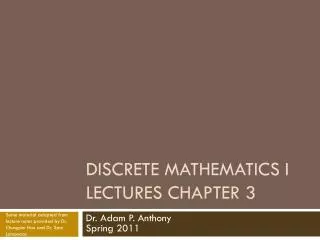
Discrete Mathematics I Chapter 11. Some material adapted from lecture notes provided by Dr. Chungsim Han and Dr. Sam Lomonaco. Dr. Adam Anthony Spring 2011. Algorithms. What is an algorithm?

E N D
Discrete Mathematics I Chapter 11 Some material adapted from lecture notes provided by Dr. Chungsim Han and Dr. Sam Lomonaco Dr. Adam Anthony Spring 2011
Algorithms • What is an algorithm? • An algorithm is a finite set of precise instructions for performing a computation or for solving a problem. • This is a rather vague definition. You will get to know a more precise and mathematically useful definition when you attend CS430. • But this one is good enough for now…
Algorithms • Properties of algorithms: • Input from a specified set, • Output from a specified set (solution), • Definiteness of every step in the computation, • Correctness of output for every possible input, • Finiteness of the number of calculation steps, • Effectiveness of each calculation step and • Generality for a class of problems.
Algorithm Examples • We will use a pseudocode to specify algorithms, which slightly reminds us of Basic and Pascal. • Example: an algorithm that finds the maximum element in a finite sequence procedure max(a1, a2, …, an: integers) max := a1 for i := 2 to n if max < ai then max := ai {max is the largest element}
Algorithm Examples • Another example: a linear search algorithm, that is, an algorithm that linearly searches a sequence for a particular element. procedure linear_search(x: integer; a1, a2, …, an: integers) i := 1 while (in and xai) i := i + 1 if in then location := i else location := 0 {location is the subscript of the term that equals x, or is zero if x is not found}
Algorithm Examples • If the terms in a sequence are ordered, a binary search algorithm is more efficient than linear search. • The binary search algorithm iteratively restricts the relevant search interval until it closes in on the position of the element to be located.
center element Algorithm Examples binary search for the letter ‘j’ search interval a c d f g h j l m o p r s u v x z
center element Algorithm Examples binary search for the letter ‘j’ search interval a c d f g h j l m o p r s u v x z
center element Algorithm Examples binary search for the letter ‘j’ search interval a c d f g h j l m o p r s u v x z
center element Algorithm Examples binary search for the letter ‘j’ search interval a c d f g h j l mo p r s u v x z
center element Algorithm Examples binary search for the letter ‘j’ search interval a c d f g h j l mo p r s u v x z found !
Algorithm Examples procedure binary_search(x: integer; a1, a2, …, an: integers) i := 1 {i is left endpoint of search interval} j := n {j is right endpoint of search interval} while (i < j) begin m := (i + j)/2 if x > am then i := m + 1 else j := m end if x = ai then location := i else location := 0 {location is the subscript of the term that equals x, or is zero if x is not found}
Complexity • In general, we are not so much interested in the time and space complexity for small inputs. • For example, while the difference in time complexity between linear and binary search is meaningless for a sequence with n = 10, it is gigantic for n = 230.
Measuring Complexity • An algorithm’s cost can be measured in terms of the number of ‘steps’ it takes to complete the work • A step is anything that takes a fixed amount of time, regardless of the input size • Arithmetic operations • Comparisons • If/Then statements • Print Statements • Etc. • Some steps in reality take longer than others, but for our analysis we will see that this doesn’t matter that much
Complexity Functions • The number of ‘steps’ needed to execute an algorithm often depends on the size of the input: • Linear_Search([1,25,33,47],33) ~ 3 ‘steps’ • Linear_Search([1,16,19,21,28,33,64,72,81], 33) ~ 6 ‘steps’ • We’ll instead express the complexity of an algorithm as a function of the size of the input N. T(N) = N (for linear search) T(N) = N2 (for other algorithms we’ll see)
Example 1 • Suppose an algorithm A requires 103n2 steps to process an input of size n. By what factor will the number of steps increase if the input size is doubled to 2n? • Answer the same question for Algorithm B which requires 2n3 steps for input size n. • Answer the same question for both, but now increase the input size to 10n.
Complexity • For example, let us assume two algorithms A and B that solve the same class of problems, both of which have an input size of n: • The time complexity of A is T(A) = 5,000n, • The time complexity of B is T(B) = 1.1n
Complexity • Comparison: time complexity of algorithms A and B Input Size Algorithm A Algorithm B n 5,000n 1.1n 10 50,000 3 100 500,000 13,781 1,000 5,000,000 2.51041 1,000,000 5109 4.81041392
Complexity • This means that algorithm B cannot be used for large inputs, while running algorithm A is still feasible. • So what is important is the growth of the complexity functions. • The growth of time and space complexity with increasing input size n is a suitable measure for the comparison of algorithms.
But wait, there’s more! • Consider the following functions: • The n2 term dominates the rest of f(n)! • Algorithm analysis typically involves finding out which term ‘dominates’ the algorithm’s complexity
Big-Oh • Definition: Let f and g be functions from the integers or the real numbers to the real numbers. • We say that f(x) is O(g(x)) if there are constants B and b such that: |f(x)| B|g(x)| whenever x > b. • In a sense, we are saying that f(x) is never greater than g(x), barring a constant factor
The Growth of Functions • When we analyze the growth of complexity functions, f(x) and g(x) are always positive. • Therefore, we can simplify the big-O requirement to • f(x) Bg(x) whenever x > b. • If we want to show that f(x) is O(g(x)), we only need to find one pair (C, k) (which is never unique).
The Growth of Functions • The idea behind the big-O notation is to establish an upper boundary for the growth of a function f(x) for large x. • This boundary is specified by a function g(x) that is usually much simpler than f(x). • We accept the constant B in the requirement • f(x) Bg(x) whenever x > b, • because B does not grow with x. • We are only interested in large x, so it is OK iff(x) > Bg(x) for x b.
The Growth of Functions • Example: • Show that f(x) = x2 + 2x + 1 is O(x2). • For x > 1 we have: • x2 + 2x + 1 x2 + 2x2 + x2 • x2 + 2x + 1 4x2 • Therefore, for B = 4 and b = 1: • f(x) Bx2 whenever x > b. • f(x) is O(x2).
The Growth of Functions • Question: If f(x) is O(x2), is it also O(x3)? • Yes. x3 grows faster than x2, so x3 grows also faster than f(x). • Therefore, we always have to find the smallest simple function g(x) for which f(x) is O(g(x)).
A Tighter Bound • Big-O complexity is important because it tells us about the worst-case • But there’s a best-case too! • Incorporating a lower bound, we get big-Theta notation: • f(x) is (g(x)) if there exist constants A, B, b such that A|g(x)| f(x) B|g(x)| for all real numbers x > b • In a sense, we are saying that f and g grow at exactly the same pace, barring constant factors
A useful observation • Given two functions f(x) and g(x), let f(x) be O(g(x)) and g(x) be O(f(x)). Then f(x) is (g(x)) and g(x) is (f(x)). • Work out on board.
Exercise 1 • Let f(x) = 2x + 1 and g(x) = x • Show that f(x) is (g(x)).
Useful Rules for Big-O • If x > 1, then 1 < x < x2 < x3 < x4 < … • If f1(x) is O(g1(x)) and f2(x) is O(g2(x)), then (f1 + f2)(x) is O(max(g1(x), g2(x))) • If f1(x) is O(g(x)) and f2(x) is O(g(x)), then(f1 + f2)(x) is O(g(x)). • If f1(x) is O(g1(x)) and f2(x) is O(g2(x)), then (f1f2)(x) is O(g1(x) g2(x)).
Exercise 2 • Let f(x) = 7x4 + 3x3 + 5 and g(x) = x4 for x ≥ 0 • Prove that f(x) is O(g(x)).
Exercise 3 • Prove that 2n3 - 6n is O(n3). • Prove that 3n4 – 4n2 + 7n – 2 is O(n4)
Exercise 4 • Let f(n) = n(n-1)/2 and g(n) = n2 for n ≥ 0. Prove that f(n) is O(g(n)).
Polynomial Order Theorem • For any polynomialf(x) = anxn + an-1xn-1 + … + a0, where a0, a1, …, an are non-zero real numbers, • f(x) is O(xn) • f(x) is Θ(xn)
Exercise 5 • Use the polynomial order theorem to show that 1 + 2 + 3 + … + n is Θ(n2).
The Growth of Functions • In practice, f(n) is the function we are analyzing and g(n) is the function that summarizes the growth of f(n) • “Popular” functions g(n) are: nlog n, 1, 2n, n2, n!, n, n3, log n • Listed from slowest to fastest growth: • 1 • log n • n • n log n • n2 • n3 • 2n • n!
The Growth of Functions • A problem that can be solved with polynomial worst-case complexity is called tractable. • Problems of higher complexity are called intractable. • Problems that no algorithm can solve are called unsolvable. • You will find out more about this in CSC 430.
Analyzing a real algorithm • What does the following algorithm compute? procedure who_knows(a1, a2, …, an: integers) m := 0 for i := 1 to n-1 for j := i + 1 to n if |ai – aj| > m then m := |ai – aj| {m is the maximum difference between any two numbers in the input sequence} • Comparisons: n-1 + n-2 + n-3 + … + 1 = (n – 1)n/2 = 0.5n2 – 0.5n • Time complexity is O(n2).
Complexity Examples • Another algorithm solving the same problem: procedure max_diff(a1, a2, …, an: integers) min := a1 max := a1 fori := 2 to n ifai < min then min := ai else if ai > max then max := ai m := max - min • Comparisons: 2n - 2 • Time complexity is O(n).
Logarithmic Orders • Logarithmic algorithms are highly desirable because logarithms grow slowly with respect to n • There are two classes that come up frequently: • log n • n*log n • The base is usually unimportant (why?) but if you must have one, 2 is a safe bet.
Exercise 6 • Prove that log(x) is O(x) • Prove that x is O(x*log(x)) • Prove that x*log(x) is O(x2).
Exercise 7 • Prove that 10x + 5x*log(x) is Θ(x*log(x))
Exercise 8 • Prove that ⎣log(n)⎦ is Θ(log(n))
Binary Representation of Integers • Let f(n) = the number of binary digits needed to represent n, for a positive integer n. Find f(n) and its order. • How many binary digits are needed to represent 325,561?