Download
1 / 37
370 likes | 678 Views
Discrete optics v.s. Integrated optics. Discrete optics:. Integrated optics:. Mirrors, lens, mechanical mounts bulky labor intensive alignment ray optics environment sensitive. Waveguide Bendable, portable Free-of-alignment wave optics robust more functionalities.

E N D
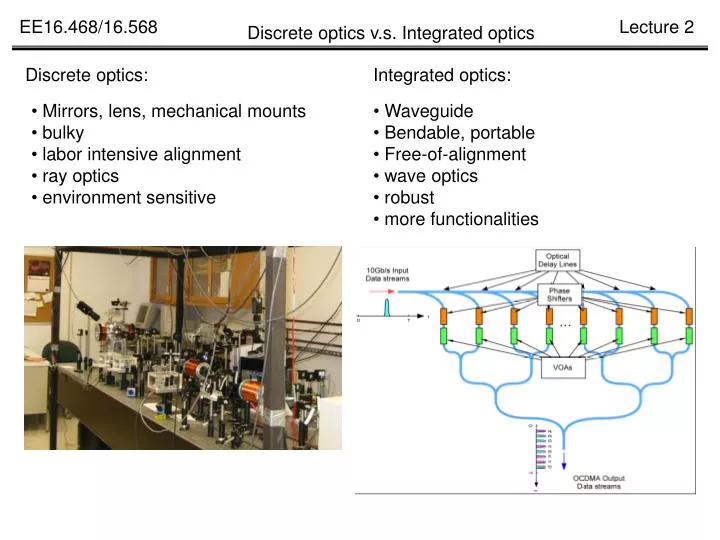
Discrete optics v.s. Integrated optics Discrete optics: Integrated optics: • Mirrors, lens, mechanical mounts • bulky • labor intensive alignment • ray optics • environment sensitive • Waveguide • Bendable, portable • Free-of-alignment • wave optics • robust • more functionalities
Discrete optics v.s. Integrated optics Applications of Integrated optics: • Transmitters and receivers, transceivers • All optical signal processing • Ultra-high speed communications (100Gbit/s), optical packet switching • RF spectrum analyzer • Smart sensors OEIC, bio/sensor Optical transceivers
Cladding, n2 Core, refractive index n1 Cladding, n2 Optical waveguides 2-D Optical waveguide x z y n2 <n1 d 1 n2 n1 n0 = 1 0 90º-1 n0*sin(0) = n1*sin(1) Numerical aperture (NA) Critical angle n1*sin(90º-1)=n2*sin(90º) cos(1)=n2/n1
Optical waveguides 2-D Optical waveguide : total acceptance angle
Optical waveguides Example 2: Calculate the acceptance angle of a core layer with index of n1= 1.468, and cladding layer of n0 = 1.447 for wavelength of 1.3m and 1.55 m. Solution: acceptance angle: Wavelength independent:
Reflections at the interface Fresnel equations n2 <n1 x z E1s E3s y z 1 1 y 1 1 n1 n1 2 n2 2 E2s n2 s-polarized beam (senkrecht: perpendicular) p-polarized beam (parallel) Trans-electric beam (TE) Trans-magnetic beam (TM)
Reflections at the interface Fresnel equations n2 <n1 x z E1s E3s y z 1 1 y 1 1 n1 n1 2 n2 2 E2s n2 Poynting vector, energy flow rate
Reflections at the interface Phase shift of reflection n2 <n1 x E1s E3s z y 1 1 n1 n2 2 E2s i.e. when because In this case, is a real number The reflection is not associated with phase shift, or phase shift is 0
Reflections at the interface Phase shift of reflection n2 <n1 E1s E3s x z 1 1 y n1 n2 2 E2s i.e. when c 1
Reflections at the interface Evanescent wave n2 <n1 x E1s z E3s y 1 1 n1 Momentum conservation n2 2 E2s Attenuated wave, penetration depth: d
Ray optics approach Optical modes C 1 A 1 1 2 d 1 B k*n1*AC – k*n1*AB = 2m AC = AB*cos(21) AB = d/sin(1)
Ray optics approach Optical modes C 1 A 1 1 2 d 1 B Propagation constant Effective index:
Ray optics approach Optical modes, considering phase shift at reflection C 1 A 1 1 2 d 1 B k*n1*AC – k*n1*AB + 2* = 2m AC = AB*cos(21) AB = d/sin(1)
Ray optics approach Optical modes C 1 A 1 1 2 d 1 B V number, normalized thickness, or normalized frequency Cut-off wavelength :
Ray optics approach Optical modes Example: estimate the number of modes • waveguide thickness 100m, free-space wavelength 1m, 49 modes
Ray optics approach Normalized waveguide equation: b: normalized propagation constant
Ray optics approach Discussion: Attenuated wave, penetration depth: D
Ray optics approach Discussions: • mode numbers v.s. index difference and wavelength • effective index difference of higher and lower order modes • mode profiles dependence on index difference and wavelength Example 1: Calculate the thickness of a core layer with index of n1= 1.468, and cladding layer of n0 = 1.447 for wavelength of 1.3m. Solution: For single mode:
Ray optics approach Normalized waveguide equation: V = 3.3 b
Ray optics approach Asymmetric waveguide n2 n1 n0 = 1 n3
Wave optics approach Maxwell equations: Dielectric materials Maxwell equations in dielectric materials: phasor
Cladding, n2 Core, refractive index n1 Cladding, n2 Wave optics approach Helmholtz Equation: Free-space solutions 2-D Optical waveguide x z y n2 <n1 d TM mode: TE mode:
Cladding, n2 Core, refractive index n1 Cladding, n2 Wave optics approach z y n2 <n1 d III n2 x d y x n1 I 0 II n2
Wave optics approach III n2 x d y x n1 I 0 II n2
Wave optics approach III n2 x d y x n1 I 0 II n2
Wave optics approach III n2 x d y x n1 I 0 II n2
Wave optics approach III n2 x d y x n1 I 0 II n2
Wave optics approach III n2 x d y x n1 I 0 II n2
Wave optics approach Graphic solution
Dispersion Dispersion Time delay
Dispersion • Material dispersion Example --- material dispersion Calculate the material dispersion effect for LED with line width of 100nm and a laser with a line width of 2nm for a fiber with dispersion coefficient of Dm = 22pskm-1nm-1 at 1310nm. Solution: for the LED for the Laser
Dispersion • Waveguide dispersion Example --- waveguide dispersion n2 = 1.48, and delta n = 0.2 percent. Calculate Dw at 1310nm. Solution: for V between 1.5 – 2.5.
Dispersion • Waveguide mode dispersion n2 n1 n0 = 1 n3 Higher order mode, Lower order mode,
Dispersion • chromatic dispersion (material plus waveduide dispersion) • material dispersion is determined by the material composition of a fiber. • waveguide dispersion is determined by the waveguide index profile of a fiber
Dispersion • Dispersion induced limitations • For RZ bit With no intersymbol interference • For NRZ bit With no intersymbol interference
Dispersion Dispersion induced limitations • Optical and Electrical Bandwidth • Bandwidth length product
Dispersion Dispersion induced limitations Example --- bit rate and bandwidth Calculate the bandwidth and length product for an optical fiber with chromatic dispersion coefficient 8pskm-1nm-1 and optical bandwidth for 10km of this kind of fiber and linewidth of 2nm. Solution: • Fiber limiting factor absorption or dispersion?