Download
1 / 14
150 likes | 297 Views
Ch. 2 Time-Domain Models of Systems. Kamen and Heck. 2.1 Input/Output Representation of Discrete-Time Systems. N-Point Moving Average y[n] = (1/N) {x[n] + x[n-1] + …+x[n-N +1] (2.1) Generalization (linear, time- invariant,causal ). 2.1.1 Exponentially Weighted Moving Average.

E N D
Ch. 2 Time-Domain Models of Systems Kamen and Heck
2.1 Input/Output Representation of Discrete-Time Systems • N-Point Moving Average • y[n] = (1/N) {x[n] + x[n-1] + …+x[n-N +1] (2.1) • Generalization (linear, time-invariant,causal)
2.1.1 Exponentially Weighted Moving Average • Let a = (1-b)/(1-bn)
2.1.2 General Class of Systems • Upper index (N-1) can be replaced by n. • Unit impulse response of the system can be obtained by letting x[n] = d[n].
Convolution Equation • The input/output representation can be rewritten with the weighting function replaced with the input response function values, h[i]. The result is called convolution.
2.2 Convolution of Discrete-Time Signals • The convolution equation can be defined for arbitrary discrete-time signals x[n] and v[n]. • The result can also be generalized for the case where • x[n] =0 for n<Q • v[n ] = 0 for n<P • In such a case the convolution result is 0 for n<P+Q.
Array Method for Computation • An array method can be used for computation of the general discrete convolution. • The columns are labeled x[Q], x[Q+1],… • The rows are labeled v[P], v[P+1]… • The array is filled in with the products of the values—then sum of elements of the backwords diagonals gives the values, y[n]. • Example 2.4 illustrates the process.
MATLAB • The matlab function conv can be used to compute discrete convolution. • Examples on page 52 and 53 illustrate the results.
Difference Equation Models • In some applications, a causal linear time-invariant discrete-time system is given by an input/output difference equation instead of an input/output convolution model. • First order linear difference equation • y[n] –ay[n-1] = -x[n]
Examples • Example 2.6 Second Order System • System can be solved recursively. • Sometimes a “complete” solution can be found recursively.
2.4 Differential Equation Models • Example 2.8 Series RC Circuit • Example 2.9 Mass-Spring-Damper System • Example 2.10 Motor with Load
2.5 Solution Of Differential Equations • Example 2.11 Series RC Circuit • Example 2.12 Using MATLAB ODE Solver • Example 2.5.2 MATLAB Symbolic MATH Solver
2.6 Convolution Representation of Continuous-Time Systems • Example 2.14 RC Circuit • 2.6.1 Graphical Approach to Convolution