Download
1 / 28
280 likes | 434 Views
A Comparison Between Bayesian Networks and Generalized Linear Models in the Indoor/Outdoor Scene Classification Problem. Overview. Introduce Scene Classification Problems Motivation for Scene Classification Kodak's JBJL Database and Features Bayesian Networks

E N D
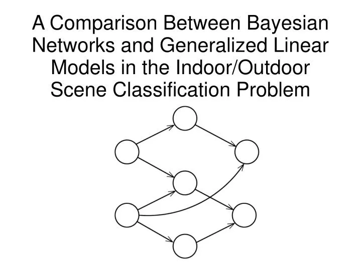
A Comparison Between Bayesian Networks and Generalized Linear Models in the Indoor/OutdoorScene Classification Problem
Overview • Introduce Scene Classification Problems • Motivation for Scene Classification • Kodak's JBJL Database and Features • Bayesian Networks • Brief Overview (description, inference, structure learning) • Classification Results • GLM • Briefer Overview • Classification Results • Comparison and Conclusion
Problem Statement: Given a set of consumer digital images, can we use a statistical model to distinguish between indoor images and outdoor images?
Motivation • Kodak • Increase visual appeal by processing based on classification • Object Recognition • Provide context information which may give clues to scale, location, identity, etc.
Procedure • Establish ground-truth for all images • Perform feature extraction and confidence/probability mapping for features • Divide images into training and testing set • Use test images to train a model to predict ground-truth • Use the model to predict ground truth for the test set • Evaluate performance
Kodak JBJL • Consumer image database • 615 indoor and 693 outdoor images • Some images are difficult for HSV to determine whether it is indoor or outdoor • Some images have indoor and outdoor parts
Features and Probability Mapping • “Low-level” Features • Ohta-space color histogram (color information) • MSAR model (texture information) • “Mid-level” Features • Grass classifier • Sky classifier • K-NN Used to Extract Probs from Features • Quantized to nearest 10% (11 states for Mid-level, 3 states for Low-level)
Stat. Model 1: Bayesian Network • Graphical Model • Variables are represented by vertices of a graph • Conditional relationships are represented by directed edges • Conditional Probability table associated with each vertex • Quantifies vertex relationships • Facilitates automated inference
Exact Inference • Model Joint Probability • Inference
Structure Learning Search Space • Space BNs • Variable-State Combination • (#States per Node) x (#Nodes) • 2178 possible • Structures • Limited to DAGs • 29281
Scoring Metric • Score a structure based on how well the data models the data • We do have an expression estimate the data given the structure • Unfortunately, the data probability is difficult to estimate
The Bayes Dirichlet Likelihood Equivalent • Can compare structures 2 at a time • What is the prior on structure? • Assume all structures are equally likely • Use #edges to penalize complex networks
Challenges • Not all structures can be considered if there is only a small amount of data. • Context dilution • Can't consider cases where CPT cannot be filled in • Finding an optimal structure is NP hard
BDe Structure For I/O Classification • Greedy algorithm with BDe scoring • Naïve Bayes Model!
Result Compared to Previous • Previous Results • Our Results
Generalized Linear Model • Outdoor and Indoor can be thought of a binary output • Logit kernel
Likelihood for GLM • Newton-Raphson • Get estimates of mean and variance (1st and 2nd derivative) • Find optimal based on estimates (Taylor Expansion) • Iterate • Generally, this quickly converges to the optimal solution
Conclusion • The newer Bayesian Network model may perform classification slightly better than GLM • BN is more computationally intensive • Unclear if there is in fact a difference • Both models have difficulty with the same images • Better to introduce new data than to use a new model • New model give (at most) marginal improvement
References • Heckerman, D. A Tutorial on Learning with Bayesian Networks. In Learning in Graphical Models, M. Jordan, ed.. MIT Press, Cambridge, MA, 1999. • Murphy, K. A Brief Introduction to Graphical Models and Bayesian Networks, http://www.cs.ubc.ca/~murphyk/Bayes/bnintro.html(viewed 4/1/08) • Lehmann, E.L. and Casella G. Theory of Point Estimation (2nd edition) • Weisberg, S. Applied Linear Regression (3rd Edition)