Download
1 / 33
330 likes | 411 Views
Screen. Cabinet. Cabinet. Lecturer’s desk. Table. Computer Storage Cabinet. Row A. 3. 4. 5. 19. 6. 18. 7. 17. 16. 8. 15. 9. 10. 11. 14. 13. 12. Row B. 1. 2. 3. 4. 23. 5. 6. 22. 21. 7. 20. 8. 9. 10. 19. 11. 18. 16. 15. 13. 12. 17. 14. Row C. 1. 2.

E N D
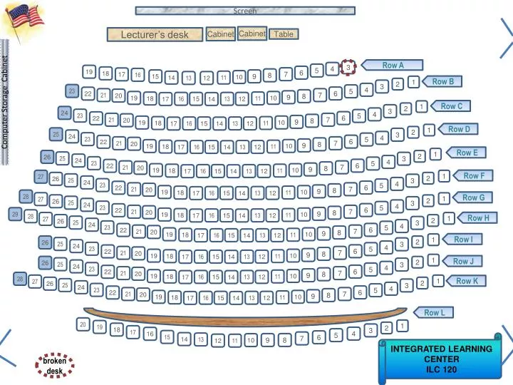
Screen Cabinet Cabinet Lecturer’s desk Table Computer Storage Cabinet Row A 3 4 5 19 6 18 7 17 16 8 15 9 10 11 14 13 12 Row B 1 2 3 4 23 5 6 22 21 7 20 8 9 10 19 11 18 16 15 13 12 17 14 Row C 1 2 3 24 4 23 5 6 22 21 7 20 8 9 10 19 11 18 16 15 13 12 17 14 Row D 1 2 25 3 24 4 23 5 6 22 21 7 20 8 9 10 19 11 18 16 15 13 12 17 14 Row E 1 26 2 25 3 24 4 23 5 6 22 21 7 20 8 9 10 19 11 18 16 15 13 12 17 14 Row F 27 1 26 2 25 3 24 4 23 5 6 22 21 7 20 8 9 10 19 11 18 16 15 13 12 17 14 28 Row G 27 1 26 2 25 3 24 4 23 5 6 22 21 7 20 8 9 29 10 19 11 18 16 15 13 12 17 14 28 Row H 27 1 26 2 25 3 24 4 23 5 6 22 21 7 20 8 9 10 19 11 18 16 15 13 12 17 14 Row I 1 26 2 25 3 24 4 23 5 6 22 21 7 20 8 9 10 19 11 18 16 15 13 12 17 14 1 Row J 26 2 25 3 24 4 23 5 6 22 21 7 20 8 9 10 19 11 18 16 15 13 12 17 14 28 27 1 Row K 26 2 25 3 24 4 23 5 6 22 21 7 20 8 9 10 19 11 18 16 15 13 12 17 14 Row L 20 1 19 2 18 3 17 4 16 5 15 6 7 14 13 INTEGRATED LEARNING CENTER ILC 120 9 8 10 12 11 broken desk
Introduction to Statistics for the Social SciencesSBS200, COMM200, GEOG200, PA200, POL200, or SOC200Lecture Section 001, Spring, 2013Room 120 Integrated Learning Center (ILC)10:00 - 10:50 Mondays, Wednesdays & Fridays. Welcome http://www.youtube.com/watch?v=oSQJP40PcGI
Please click in My last name starts with a letter somewhere between A. A – D B. E – L C. M – R D. S – Z Please hand in your homework
Use this as your study guide By the end of lecture today2/25/13 • Probability of an event • Complement of an event; Union of two events • Intersection of two events; Mutually exclusive events • Collectively exhaustive events • Conditional probability • Connecting raw scores, z scores and probabilityConnecting probability, proportion and area of curve • Law of Large Numbers • Central Limit Theorem • Three propositions • True mean 2) Standard Error of Mean 3) Normal Shape • Calculating Confidence Intervals http://onlinestatbook.com/stat_sim/sampling_dist/index.html http://www.youtube.com/watch?v=ne6tB2KiZuk
Schedule of readings Before next exam (This Friday - March 1st) Please read chapters 5, 6, & 8 in Ha & Ha Please read Chapters 10, 11, 12 and 14 in Plous Chapter 10: The Representativeness Heuristic Chapter 11: The Availability Heuristic Chapter 12: Probability and Risk Chapter 14: The Perception of Randomness Study Guide is online
Lab sessions Labs continue Review for Exam 1
Homework due – Wednesday (February 27th) • On class website: • Please print and complete homework worksheet #14 • Confidence Intervals
Union versus Intersection ∩ P(A B) Union of two events means Event A or Event B will happen Intersection of two events means Event A and Event B will happen Also called a “joint probability” P(A ∩ B)
The union of two events: all outcomes in the sample space S that are contained either in event Aor in event Bor both (denoted A B or “A or B”). may be read as “or” since one or the other or both events may occur.
The union of two events: all outcomes contained either in event Aor in event Bor both (denoted A B or “A or B”). What is probability of drawing a red card or a queen? what is Q R? It is the possibility of drawing either a queen (4 ways) or a red card (26 ways) or both (2 ways).
Probability of picking a Queen Probability of picking a Red 26/52 4/52 P(Q) = 4/52(4 queens in a deck) 2/52 P(R) = 26/52 (26 red cards in a deck) P(Q R) = 2/52 (2 red queens in a deck) Probability of picking both R and Q When you add the P(A) and P(B) together, you count the P(A and B) twice. So, you have to subtract P(A B) to avoid over-stating the probability. P(Q R) = P(Q) + P(R) – P(Q R) = 4/52 + 26/52 – 2/52 = 28/52 = .5385 or 53.85%
Union versus Intersection ∩ P(A B) Union of two events means Event A or Event B will happen Intersection of two events means Event A and Event B will happen Also called a “joint probability” P(A ∩ B)
The intersection of two events: all outcomes contained in both event A and event B(denoted A B or “A and B”) What is probability of drawing red queen? what is Q R? It is the possibility of drawing both a queen and a red card (2 ways).
If two events are mutually exclusive (or disjoint) their intersection is a null set (and we can use the “Special Law of Addition”) P(A ∩ B) = 0 Intersection of two events means Event A and Event B will happen Examples: mutually exclusive If A = Poodles If B = Labradors Poodles and Labs:Mutually Exclusive (assuming purebred)
If two events are mutually exclusive (or disjoint) their intersection is a null set (and we can use the “Special Law of Addition”) P(A ∩ B) = 0 ∩ Dog Pound P(A B) = P(A) +P(B) Intersection of two events means Event A and Event B will happen Examples: If A = Poodles If B = Labradors (let’s say 10% of dogs are poodles) (let’s say 15% of dogs are labs) What’s the probability of picking a poodle or a lab at random from pound? P(poodle or lab) = P(poodle) + P(lab) P(poodle or lab) = (.10) + (.15) = (.25) Poodles and Labs:Mutually Exclusive (assuming purebred)
Conditional Probabilities Probability that A has occurred given that B has occurred Denoted P(A | B): The vertical line “ | ” is read as “given.” P(A ∩ B) P(A | B) = P(B) The sample space is restricted to B, an event that has occurred. A B is the part of B that is also in A. The ratio of the relative size of A B to B is P(A | B).
Conditional Probabilities Probability that A has occurred given that B has occurred Of the population aged 16 – 21 and not in college: P(U) = .1350 P(ND) = .2905 P(UND) = .0532 What is the conditional probability that a member of this population is unemployed, given that the person has no diploma? .0532 P(A ∩ B) .1831 = P(A | B) = = .2905 P(B) or 18.31%
Conditional Probabilities Probability that A has occurred given that B has occurred Of the population aged 16 – 21 and not in college: P(U) = .1350 P(ND) = .2905 P(UND) = .0532 What is the conditional probability that a member of this population is unemployed, given that the person has no diploma? .0532 P(A ∩ B) .1831 = P(A | B) = = .2905 P(B) or 18.31%
Standard Error of the Mean (SEM) Remember confidence intervals? Revisit Confidence Intervals Confidence Intervals (based on z): We are using this to estimate a value such as a population mean, with a known degree of certainty with a range of values • The interval refers to possible values of the population mean. • We can be reasonably confident that the population mean • falls in this range (90%, 95%, or 99% confident) • In the long run, series of intervals, like the one we • figured out will describe the population mean about 95% • of the time. Greater confidence implies loss of precision.(95% confidence is most often used) Can actually generate CI for any confidence level you want – these are just the most common
? ? Mean = 50Standard deviation = 10 Find the scores for the middle 95% 95% x = mean ± (z)(standard deviation) 30.4 69.6 .9500 Please note: We will be using this same logic for “confidence intervals” .4750 .4750 ? 1) Go to z table - find z score for for area .4750 z = 1.96 2) x = mean + (z)(standard deviation) x = 50 + (-1.96)(10) x = 30.4 30.4 3) x = mean + (z)(standard deviation) x = 50 + (1.96)(10) x = 69.6 69.6 Scores 30.4 - 69.6 capture the middle 95% of the curve
? ? Mean = 50Standard deviation = 10 n = 100 s.e.m. = 1 Confidence intervals σ 95% standard error of the mean = Find the scores for the middle 95% n √ 48.04 51.96 For “confidence intervals” same logic – same z-score But - we’ll replace standard deviation with the standard error of the mean .9500 .4750 .4750 ? 10 = 100 √ x = mean ± (z)(s.e.m.) x = 50 + (1.96)(1) x = 51.96 x = 50 + (-1.96)(1) x = 48.04 95% Confidence Interval is captured by the scores 48.04 – 51.96
Confidence intervals ? ? σ standard error of the mean 95% = n √ Mean = 50 Standard error mean = 10 Hint always draw a picture! Tell me the scores associated that border exactly the middle 95% of the curve We know this raw score = mean ± (z score)(standard deviation) Construct a 95 percent confidence interval around the mean Similar, but uses standard error the mean raw score = mean ± (z score)(standard error of the mean)
Law of large numbers: As the number of measurements increases the data becomes more stable and a better approximation of the true (theoretical) probability As the number of observations (n) increases or the number of times the experiment is performed, the estimate will become more accurate.
Law of large numbers: As the number of measurements increases the data becomes more stable and a better approximation of the true signal (e.g. mean) As the number of observations (n) increases or the number of times the experiment is performed, the signal will become more clear (static cancels out) With only a few people any little error is noticed (becomes exaggerated when we look at whole group) With many people any little error is corrected (becomes minimized when we look at whole group) http://www.youtube.com/watch?v=ne6tB2KiZuk
Sampling distributions of sample means versus frequency distributions of individual scores Distribution of raw scores: is an empirical probability distribution of the values from a sample of raw scores from a population Eugene X X X X X X X X X X X X X X X X X X X X X X X X X X X X X X X X • Frequency distributions of individual scores • derived empirically • we are plotting raw data • this is a single sample Melvin X X X X X X X X X X X X Take a single score x Repeat over and over x x x Population x x x x
Sampling distribution: is a theoretical probability distribution of • the possible values of some sample statistic that would • occur if we were to draw an infinite number of same-sized • samples from a population important note: “fixed n” • Sampling distributions of sample means • theoretical distribution • we are plotting means of samples Take sample – get mean Repeat over and over Population
Sampling distribution: is a theoretical probability distribution of • the possible values of some sample statistic that would • occur if we were to draw an infinite number of same-sized • samples from a population important note: “fixed n” • Sampling distributions of sample means • theoretical distribution • we are plotting means of samples Take sample – get mean Repeat over and over Population Distribution of means of samples
Sampling distribution: is a theoretical probability distribution of • the possible values of some sample statistic that would • occur if we were to draw an infinite number of same-sized • samples from a population Eugene • Frequency distributions of individual scores • derived empirically • we are plotting raw data • this is a single sample X X X X X X X Melvin X X X X X X X X X X X X X X X X X X X X X X X X X X X X X X X X X X X X X • Sampling distributions sample means • theoretical distribution • we are plotting means of samples 23rd sample 2nd sample
X X X X X X X X X X X X X X X X X X X X X X X X X X X X X X X X X X X X X X X Sampling distribution for continuous distributions • Central Limit Theorem: If random samples of a fixed N are drawn • from any population (regardless of the shape of the • population distribution), as N becomes larger, the • distribution of sample means approaches normality, with • the overall mean approaching the theoretical population • mean. Distribution of Raw Scores Sampling Distribution of Sample means Melvin 23rd sample Eugene X X X X X 2nd sample
Thank you! See you next time!!