Download
1 / 20
200 likes | 347 Views
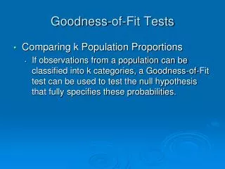
Goodness of Fit Test for Proportions of Multinomial Population. Chi-square distribution Hypotheses test/Goodness of fit test. Chi-square distribution. With 2 degrees of freedom. With 5 degrees of freedom. With 10 degrees of freedom. 0. Chi-Square Distribution.

E N D
Goodness of Fit Test for Proportions of Multinomial Population Chi-square distribution Hypotheses test/Goodness of fit test
Chi-square distribution With 2 degrees of freedom With 5 degrees of freedom With 10 degrees of freedom 0
Chi-Square Distribution • We will use the notation to denote the value for the chi-square distribution that provides an area of a to the right of the stated value. • For example, there is a .95 probability of obtaining a c2 (chi-square) value such that
Our value For 9 d.f. and a = .975 Selected Values from the Chi-Square Distribution Table
.025 Area in Upper Tail = .975 2 0 2.700
Our value For 9 d.f. and a = .025 Selected Values from the Chi-Square Distribution Table
Area in Upper Tail = .025 2 0 19.023
Our value For 9 d.f. and a = .10 Selected Values from the Chi-Square Distribution Table
Area in Upper Tail = .10 2 14.684 0
For 9 d.f. and =16.919, = .05 • For 8 d.f. and =3.49, = .90 • For 6 d.f. and =16.812, = .01 • For 10 d.f. and =18.9, = between .05 and .025
Hypothesis (Goodness of Fit) Testfor Proportions of a Multinomial Population This is simply a hypothesis test to see if the hypothesized population proportions agree with the observed population proportions from our sample. 1. Set up the null and alternative hypotheses. 2. Select a random sample and record the observed frequency, fi , for each of the k categories. 3. Assuming H0 is true, compute the expected frequency, ei , in each category by multiplying the category probability by the sample size.
Hypothesis (Goodness of Fit) Testfor Proportions of a Multinomial Population 4. Compute the value of the test statistic. where: fi = observed frequency for category i ei = expected frequency for category i k = number of categories Note: The test statistic has a chi-square distribution with k – 1 df provided that the expected frequencies are 5 or more for all categories.
Reject H0 if Hypothesis (Goodness of Fit) Testfor Proportions of a Multinomial Population 5. Rejection rule: Reject H0 if p-value <a p-value approach: Critical value approach: where is the significance level and there are k - 1 degrees of freedom
Multinomial Distribution Goodness of Fit Test • Example: Finger Lakes Homes (A) Finger Lakes Homes manufactures four models of prefabricated homes, a two-story colonial, a log cabin, a split-level, and an A-frame. To help in production planning, management would like to determine if previous customer purchases indicate that there is a preference in the style selected.
Multinomial Distribution Goodness of Fit Test • Example: Finger Lakes Homes (A) The number of homes sold of each model for 100 sales over the past two years is shown below. Split- A- Model Colonial Log Level Frame # Sold 30 20 35 15
Multinomial Distribution Goodness of Fit Test • Hypotheses H0: pC = pL = pS = pA = .25 Ha: The population proportions are not pC = .25, pL = .25, pS = .25, and pA = .25 where: pC = population proportion that purchase a colonial pL = population proportion that purchase a log cabin pS = population proportion that purchase a split-level pA = population proportion that purchase an A-frame
Multinomial Distribution Goodness of Fit Test • Rejection Rule Reject H0 if p-value < .05 or c2 > 7.815. With = .05 and k - 1 = 4 - 1 = 3 degrees of freedom Do Not Reject H0 Reject H0 2 7.815
Multinomial Distribution Goodness of Fit Test • Expected Frequencies • Test Statistic • e1 = .25(100) = 25 e2 = .25(100) = 25 e3 = .25(100) = 25 e4 = .25(100) = 25 = 1 + 1 + 4 + 4 = 10
Multinomial Distribution Goodness of Fit Test • Conclusion Using the p-Value Approach Area in Upper Tail .10 .05 .025 .01 .005 c2 Value (df = 3) 6.251 7.815 9.348 11.345 12.838 Because c2 = 10 is between 9.348 and 11.345, the area in the upper tail of the distribution is between .025 and .01. The p-value <a . We can reject the null hypothesis.
Multinomial Distribution Goodness of Fit Test • Conclusion Using the Critical Value Approach c2 = 10 > 7.815 We reject, at the .05 level of significance, the assumption that there is no home style preference.