Functional Methods for Testing Data

1. Functional Methods for Testing Data

2. The data • Each person a = 1,…,N • responds to each item i = 1,…,n • and makes a binary response = uai , where 0 indicates “wrong” and 1 indicates “right”. • We want to estimate Pai = the probability of person a getting item i right.

3. The model • The response space is an n-dimensional unit hypercube. The data vectors {ua1,…,uan} are on the corners. • The vectors of correct response probabilities {Pa1,…,Pan}fall along a smooth curve in response space, the response manifold. • This manifold is, in principle, identifiable from the data, is therefore not a latent trait.

4. Item response functions • We can define a smooth charting function that maps each point on the response manifold to a corresponding real number θ. E.g.: arc length. • In this way we establish a metric defining positions on this manifold. • Pi(θ) is the success probability for item i of all those at position θ. This is a smooth function of θ : The item response function for item i.

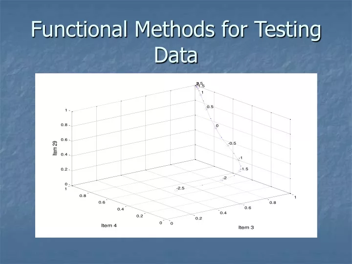
5. Three items from an Intro Psych test • The response manifold for 3 test items: 3, 4, and 29. • The curve indicates the possible values of Pai = Pi (θ) . • The circles correspond to 11 fixed values of θ.

6. What does “smooth” mean? If θ has a standard normal distribution, then experience indicates that usually: • The function Pi (θ) is monotonic. • It has slopes near 0 for extreme θvalues. • The lower asymptote is positive, and the upper asymptote is one. • There is only one inflection point.

7. The three-parameter logistic item response function is smooth

8. The challenges • Let the item response functions take whatever shapes are supported by the data. • But control their smoothness in this sense. • Constrain the function values to lie within [0,1]. • We want a smooth derivative, too, for the item information function.

9. We actually estimate Wi(θ) = log [Pi (θ) /Qi (θ)], where Qi (θ) = 1 – Pi (θ). “Smooth” in terms of Wi (θ) means linear behavior for extreme θ, with small slope on the left and larger positive slope on the right. The log-odds transformation deals with the [0,1] constraint

10. The log-odds transformation of a 3PL item response function

11. A three-dimensional model for a smooth log-odds function The function log(e θ+1) has the desired behavior at the extremes. The other two terms add vertical shift and tilt as required.

12. Comparing the 3D model and the 3PL log-odds functions

13. B-spline expansions for W(θ) But, in fact, we will actually estimate our log-odds functions by • expanding W(θ) in terms of a set of K B-spline basis functions, while • smoothing these expansions towards these simpler three-dimensional models.

14. Fitting the data We use maximum marginal likelihood estimation, using the EM algorithm to maximize where g(θ) is a prior density on θ, often taken to be the standard normal. Maximization is with respect to the nK coefficients defining the B-spline expansions of the log-odds functions.

15. What about smoothness? • We have defined smoothness here in a less orthodox fashion; It isn’t defined only in terms of the second derivative. • Instead, we define smooth in terms of the size of

16. How did you come up with this? • If W(θ) conforms exactly to the three-dimensional smooth model, then LW(θ)= 0. • In other words, if then

17. Our strategy is to define a low-dimensional family of prototype functions that capture what we mean by “smooth.” • Then we represent this family by a linear differential equation. • This differential equation defines a measure of “roughness”, which we penalize. • The more we penalize this kind of roughness, the more we force the fitted functions to be smooth.

18. In general, if we begin with a linear model of dimension m, we can find a linear differential equation of order m such that all versions of this model will satisfy: DmW(θ) = b0 (θ) W(θ)+ b1 (θ) DW(θ)+ … + bm-1 (θ) Dm-1W(θ) for some choice of coefficient functions bj(θ). • We change the equation to a roughness penalty by converting it to operator form: LW(θ) = b0 (θ) W(θ)+ b1 (θ) DW(θ)+…+ bm-1 (θ) Dm-1W (θ) + DmW(θ) = 0.

19. The roughness-penalty measures the departure ofW(θ) from this smooth model.

20. Roughness-penalized log marginal likelihood Consequently, we actually maximize Smoothing parameter λ controls the amount of smoothness in the W(θ)‘s; the larger it is, the more these will look like the three-dimensional versions.

21. Some examples • Here are three estimates of the item response functions for items 3, 4, 29, and 96 for an introductory psychology test • The test had 100 items, and was given to 379 students. • Each function W(θ) is defined by an expansion in terms of 13 B-spline basis functions.

22. λ=0

23. λ=0.01

24. λ=50

25. What does θmean? • We have fallen into the habit of calling θa “latent trait score”. • Actually, it is the value of a function that is chosen more or less arbitrarily to map position along the response manifold. • The assumption of a standard normal distribution is pure convention. • We can choose otherwise.

26. What charting functions would be more useful? • Three choices of charting functions are especially interesting, and none are “latent” in any sense. • Each leads to interesting diagnostic statistics and graphics.

27. The arc length charting • Arc length s measures the Euclidean distance traveled along the manifold from its origin at θ0 to a given position θ:

28. Item discrimination in arc length metric One useful property of arc length is Each squared item discrimination is a proportion total test discrimination, and therefore has a familiar frame of reference.

29. Expected score charting Assuming that expected score is monotonically related to θ, (there aren’t too many items like 96), then Provides a metric that is familiar to users and easy for them to interpret. Expected score is already used extensively as a basis for assessing differential item functioning (DIF).

30. ACT Math test for males and females • Three items from a 60 item math test. • Around 2000 examinees. • The male and female response manifolds differ.

31. Differential item functioning for an ACT Math test item

32. Total change charting The following total change in probability of success measure is closely related to arc length:

33. Some general lessons • Fitting functional models to non-functional data is relatively straight-forward. • But we do need to transform constrained functions into unconstrained versions. • We can define smoothness or roughness in customized ways that capture the default or baseline behavior of our estimated functions.

34. “Latent trait models” aren’t really latent at all. • They express the idea of a one-dimensional subspace for modeling the data. • Differential geometry gives us the appropriate mathematical tools. • There is room for creativity in choosing charting functions.

35. Looking ahead • There is an intimate connection between designer roughness penalties and the estimation of differential equations from data. • We will use discrete data to estimate a differential equation that describes the data.

36. References More technical details on fitting test data with functional models are in Rossi, N., Wang, X. and Ramsay, J. O. (2002) Nonparametric item response function estimates with the EM algorithm. Journal of Educational and Behavioral Statistics, 27, 291-317.