Download
1 / 10
100 likes | 274 Views
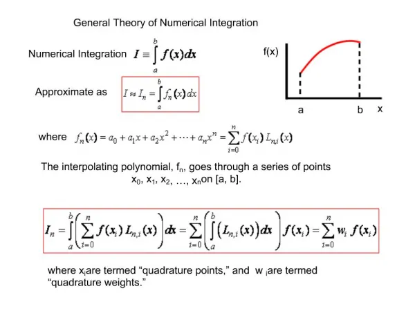
Revisiting Numerical Integration: Getting More from Fewer Points. David Sklar San Francisco State University dsklar@sfsu.edu. Bruce Cohen Lowell High School, SFUSD bic@cgl.ucsf.edu http://www.cgl.ucsf.edu/home/bic. Asilomar - December 2007. Ver. 3.00. Romberg Integration.

E N D
Revisiting Numerical Integration: Getting More from Fewer Points David Sklar San Francisco State University dsklar@sfsu.edu Bruce Cohen Lowell High School, SFUSD bic@cgl.ucsf.edu http://www.cgl.ucsf.edu/home/bic Asilomar - December 2007 Ver. 3.00
Romberg Integration The method arises from a technique called Richardson extrapolation which can be used whenever the error E(h) can be expanded in a series of the form We’ll illustrate Richardson’s technique by applying it to the trapezoidal rule. In fact we can show that if f can be expanded in a Taylor series on each subinterval then E can be expanded in a series of the form
To implement the method we don’t need to know the coefficients, we need only know that they exist. Assume that we have computed trapezoidal estimates for I for h, h/2, h/4, h/8, so we have Just looking at the first two we have Romberg Integration We can eliminate the h2 term by multiplying the second by 22 and subtracting the first giving Which we can rewrite as
Which is in the form Romberg Integration The last equation is equivalent to T2(h) is an estimate for I with an error that is O(h4)
We can repeat the process beginning with And get a new estimate with Where for each estimate we have Romberg Integration Continuing in this way we get a sequence of estimates for the integral I
5.858234 5.841100 5.836813 5.835740 Romberg Integration -- An example To see how Romberg integration works we organize our estimates into an array as follows We place our trapezoidal estimates in the first column. The first estimate corresponds to a partition of [1, 3] into 4 subintervals, an h value of ½. Accuracy improves as we move down the column The accuracy increases as we move down and as we move to the right. 5.835388 Next we perform Romberg integration for a familiar example. 5.835384 5.835384 5.835382 5.835382 5.835382
5.835388 5.835384 5.835384 5.85823385920 5.858234 5.84110042206 5.835382 5.835382 5.835382 5.841100 5.83681259147 5.836813 5.83574034752 5.835740 Romberg Integration -- An example We can improve our Romberg result if we start with more precise (though quite inaccurate) trapezoidal estimates in the first column. The averaging method used to get the more accurate estimates involves the subtraction of nearly equal numbers which can lead to precision loss as the computation progresses. The distinction between precision and accuracy in computation is important in practical numerical analysis. 5.83538927635 5.83538331460 5.83538291715 5.83538293287 5.83538290742 5.83538290726 Note: The correct value to 12 significant digits is 5.83538290725
Gaussian Quadrature In Gaussian quadrature the approximation to the integral is also a weighted sum of function values. The evaluation points (which are not equally spaced ) and weights are chosen to provide a very efficient estimate. One way to implement Gaussian quadrature is to first transform the integral to an integral from –1 to 1, and then, for appropriate numbers of points n, get the gauss points and weights from the table. For our example we have
Bibliography 1. M. Abramowitz, I. Stegun, Handbook of Mathematical Functions, Dover, New York, 1965 2. R. Burden, J. Faires, Numerical Analysis, 7th Edition, Brooks/Cole, 2001 3. F. B. Hildebrand, Introduction to Numerical Analysis, McGraw-Hill, New York, 1956 4. http://numericalmethods.eng.usf.edu/anecdotes/romberg.doc 5. http://www-history.mcs.st-andrews.ac.uk/Biographies/ • R Development Core Team, R: A language and environment for statistical • computing, R Foundation for Statistical Computing, Vienna, Austria, • 2006, <http://www.R-project.org> • L. F. Richardson and J. L. Gaunt, The deferred approach to the limit, • Philosophical Transactions of the Royal Society of London 226A, 1927 • W. Romberg, W. (1955), "Vereinfachte numerische Integration", Norske • Videnskabers Selskab Forhandlinger (Trondheim)28(7), 1955